Rank two Artin–Schelter regular algebras from noncommuting derivations

Vincent Beck; César Lecoutre

doi:10.4171/jncg/679

JournalsjncgVol. 20, No. 4pp. 1225–1277

Rank two Artin–Schelter regular algebras from noncommuting derivations

Vincent Beck
Université d’Orléans, France
César Lecoutre
Université Clermont Auvergne, Aubière, France

Download PDF

This article is published open access under our Subscribe to Open model.

Abstract

If

Δ

and

Γ

are two derivations of a commutative algebra

A

such that

Δ Γ - Γ Δ = Δ

is locally nilpotent, one can endow

A

with a new product

*

whose filtered semiclassical limit is the Poisson structure

Δ \land Γ .

In this article, we first study these (Poisson) algebras from an algebraic point of view, and when

A

is a polynomial algebra, we investigate their homological properties. In particular, when the derivations

Δ

and

Γ

are linear, the algebras

(A, *)

provide, in each dimension at least four, new examples of multiparameter families of Artin–Schelter regular algebras. These algebras are deformations of Poisson algebras

(A, Δ \land Γ)

of rank two, thus explaining the title of the article. Assuming furthermore a technical condition on

Γ,

we show that the algebra

(A, *)

is Calabi–Yau if and only if the trace of

Γ

is equal to

1

if and only if the Poisson algebra

(A, Δ \land Γ)

is unimodular. Since the trace of

Γ

is a linear function of the parameters, the algebras

(A, *)

also provide, in each dimension at least four, new examples of multiparameter families of Calabi–Yau algebras.

Introduction

The philosophy behind noncommutative projective algebraic geometry [24

D. Rogalski, Noncommutative projective geometry. Math. Sci. Res. Inst. Publ. 64 (2016), 13–70 Zbl 1386.14016 MR 3618472

] is to study noncommutative version of the projective spaces

ℙ^{n}

by describing suitable noncommutative algebras that would be thought of as their homogeneous coordinates rings: the so-called Artin–Schelter regular algebras (AS regular algebras for short) [2

M. Artin and W. F. Schelter, Graded algebras of global dimension

3

. Adv. Math. 66 (1987), no. 2, 171–216 Zbl 0633.16001 MR 0917738

]. Numerous examples of AS regular algebras are known, but a complete classification is achieved only up to projective dimension

2 .

The work of Pym [22

B. Pym, Quantum deformations of projective three-space. Adv. Math. 281 (2015), 1216–1241 Zbl 1338.14007 MR 3366864

] provides a partial answer in dimension

3

by focusing on a classification of graded Calabi–Yau algebras [10

V. Ginzburg, Calabi–Yau algebras. [v1] 2006, [v3] 2007, arXiv:math/0612139v3

] that are flat deformations of

ℂ [x_{0}, x_{1}, x_{2}, x_{3}] .

In [16

C. Lecoutre and S. J. Sierra, A new family of Poisson algebras and their deformations. Nagoya Math. J. 233 (2019), 32–86 Zbl 1461.16032 MR 3901632

], Sierra and the second author introduced a family of AS regular algebras

R (n, a)

of Gel’fand–Kirillov dimension

n + 1

indexed by a scalar

a .

The authors proved that for any integer

n \geq 0,

there exists a unique scalar

a

such that the algebra

R (n, a)

is Calabi–Yau. This is of particular interest since it explains a specific choice of parameter made in the exceptional component

E (3)

of Pym’s classification [22

B. Pym, Quantum deformations of projective three-space. Adv. Math. 281 (2015), 1216–1241 Zbl 1338.14007 MR 3366864

].

Back to the algebra

R (n, a),

the parameter

n + 1

can be interpreted as the index of nilpotency of a maximal Jordan block seen as the restriction to degree one polynomials of a locally nilpotent derivation

Δ

of a polynomial algebra in

n + 1

variables. The construction of

R (n, a)

relies on a second derivation

Γ

such that

Δ Γ - Γ Δ = Δ

together with a deformation formula of Coll, Gerstenhaber, and Giaquinto [5

V. Coll, M. Gerstenhaber, and A. Giaquinto, An explicit deformation formula with noncommuting derivations. In Ring theory 1989. In honor of S. A. Amitsur (Proc. Sympos. Workshop, Jerusalem, Israel, 1988/89), pp. 396–403, Israel Math. Conf. Proc. 1, Weizmann, Jerusalem, 1989 Zbl 0684.16016 MR 1029329

]. The aim of this article is to investigate the following natural generalization: what are the possible algebras arising from this construction by relaxing the conditions on

Δ

? The case of homogeneous locally nilpotent derivations

Δ

of a polynomial ring whose canonical Jordan normal form acting on the set of degree one polynomials is not a maximal block will be of particular interest. In this situation, we obtain a wide family of non-isomorphic AS regular algebras in each dimension since the Jordan type of

Δ

must be preserved by isomorphism (Theorem 5.9). Among them, we describe a family of Calabi–Yau algebras indexed by

r - 1

scalar parameters, where

r

is the number of blocks in the canonical Jordan normal form of

Δ

(the algebras studied in [16

C. Lecoutre and S. J. Sierra, A new family of Poisson algebras and their deformations. Nagoya Math. J. 233 (2019), 32–86 Zbl 1461.16032 MR 3901632

] correspond to the case

r = 1

).

This article is divided into eight sections. In Section 1, we present the general construction of a Poisson algebra

A_{(Δ, Γ)}

and an associative algebra

R_{(Δ, Γ)}

associated with a pair of derivations

(Δ, Γ)

of a commutative algebra

A

such that

Δ Γ - Γ Δ = Δ

is locally nilpotent. Such a pair of derivations will be called a solvable pair. Section 2 is devoted to the study of general algebraic properties of

A_{(Δ, Γ)}

and

R_{(Δ, Γ)} .

A lot of examples of solvable pairs are given. Moreover, we compute the (Poisson) center in many cases (Lemma 2.9) and exhibit examples of important Poisson derivations of

A_{(Δ, Γ)}

and automorphisms of

R_{(Δ, Γ)}

(see Lemma 2.15 and Theorem 2.17). Furthermore, we remark that the natural filtration associated with the locally nilpotent derivation

Δ

is compatible with both the Poisson structure of

A_{(Δ, Γ)}

and the associative structure of

R_{(Δ, Γ)} .

This filtration is presented and studied in Section 2.4; it will be one of our main tools to prove a lot of results in this article. In the general situation, not much can be said about normal elements. However, among them, we identify and study a significant subset consisting of the so-called strongly normal elements (Definition 2.30) which will be of particular interest later in this article. To end Section 2, we observe that up to localization, the Poisson algebra

A_{(Δ, Γ)}

and the algebra

R_{(Δ, Γ)}

are particularly nice: they are isomorphic to (Poisson) Ore extensions over (a localization of) the kernel of

Δ,

thanks to the local slice construction.

The rest of the article is devoted to the case where the solvable pair is defined on a polynomial algebra

A .

In Section 3, the rank of a non-abelian Poisson algebra

A_{(Δ, Γ)}

is shown to be equal to two. Section 4 deals with the case of homogeneous derivations

Δ

and

Γ .

In this situation, both the Poisson center of

A_{(Δ, Γ)}

and the center of

R_{(Δ, Γ)}

are characterized (Corollary 4.8). Moreover, we construct a finer filtration than the previous one, having the benefit that the associated graded algebra is a polynomial algebra. In Section 5, we show that the algebra

R_{(Δ, Γ)}

is AS regular, and we characterize the (Poisson) normal elements: they are precisely the strongly normal elements introduced in Section 2. Moreover, we prove that the Jordan type of

Δ

is an invariant of both

A_{(Δ, Γ)}

and

R_{(Δ, Γ)} .

In Sections 6 and 7, we focus on the case where

Γ

is diagonalizable. In this situation, we are able to determine the linear Poisson derivations when

Γ

is generic. We also provide a presentation of

R_{(Δ, Γ)}

by generators and relations. In the last section, we study when our algebras (resp. Poisson algebras) are Calabi–Yau (resp. unimodular); see Corollary 8.12. Finally, the article ends with appendices which recap some of the results frequently used in the article, in particular it explains the structure of the graded ring for the finer of the filtrations we study. In this article, we always assume that

𝕜

is a field of characteristic zero.

1. A deformation formula for noncommuting derivations

Let

A

be a commutative

𝕜 -

algebra and

Δ, Γ

be two derivations of

A

such that

[Δ, Γ] = Δ Γ - Γ Δ = Δ .

It is easily verified that the biderivation

{-, -} = Δ \land Γ

satisfies the Jacobi identity and hence is a Poisson bracket on

A .

More precisely, we have

(1.1)

{f, g} = Δ (f) Γ (g) - Δ (g) Γ (f)

for any

f, g \in A .

Moreover, if

Δ

is locally nilpotent, by setting for any

f, g \in A,

(1.2)

f * g = \sum_{i \geq 0} Δ^{i} (f) (\binom{Γ}{i}) (g) = f g + Δ (f) Γ (g) + \sum_{i \geq 2} Δ^{i} (f) (\binom{Γ}{i}) (g),

where

(\binom{Γ}{i}) = \frac{1}{i!} Γ \circ (Γ - id) \circ \dots \circ (Γ - (i - 1) id),

we define an associative product on

A;

see [5

V. Coll, M. Gerstenhaber, and A. Giaquinto, An explicit deformation formula with noncommuting derivations. In Ring theory 1989. In honor of S. A. Amitsur (Proc. Sympos. Workshop, Jerusalem, Israel, 1988/89), pp. 396–403, Israel Math. Conf. Proc. 1, Weizmann, Jerusalem, 1989 Zbl 0684.16016 MR 1029329

] for the formal version and [22

B. Pym, Quantum deformations of projective three-space. Adv. Math. 281 (2015), 1216–1241 Zbl 1338.14007 MR 3366864

, Lemma 3.3] for the algebraic version. We set

$A = A_{(Δ, Γ)} = (A, {-, -}),$
$R = R_{(Δ, Γ)} = (A, *) .$

The algebra

R

is a deformation of the Poisson algebra

A

in the following sense. Consider

A [t]

as an algebra over

𝕜 [t]

and define

f *_{t} g = \sum_{i \geq 0} t^{i} Δ^{i} (f) (\binom{Γ}{i}) (g) .

Then

A_{t} = (A [t], *_{t})

is an associative algebra over

𝕜 [t]

such that

$A_{t} / (t - 1) A_{t} ≅ R,$
$A_{t} / t A_{t}$ is commutative and can be endowed with a Poisson structure given by

${f + t A_{t}, g + t A_{t}} = \frac{f *_{t} g - g *_{t} f}{t} + t A_{t},$
$A_{t} / t A_{t}$ and $A$ are isomorphic as Poisson algebras.

Therefore, the Poisson algebra

A_{(Δ, Γ)}

is the commutative fiber version of the semiclassical limit of

R_{(Δ, Γ)}

in the sense of [11

K. R. Goodearl, Semiclassical limits of quantized coordinate rings. In D. Van Huynh and S. R. López-Permouth (eds.), Advances in ring theory, pp. 165–204, Trends Math., Birkhäuser, Basel, 2010 Zbl 1202.16027 MR 2664671

, Section 2.1].

Example 1.3.

For

A = 𝕜 [X_{0}, \dots, X_{n}]

and the derivations

Δ (X_{i}) = X_{i - 1}

(

X_{- 1} = 0

) and

Γ (X_{i}) = (a + i) X_{i}

(

a \in 𝕜

), the (Poisson) algebras obtained by formulae (1.1) and (1.2) have been studied in [16

C. Lecoutre and S. J. Sierra, A new family of Poisson algebras and their deformations. Nagoya Math. J. 233 (2019), 32–86 Zbl 1461.16032 MR 3901632

] where they are denoted by

A (n, a)

and

R (n, a) .

In this article, our aim is to generalize the results of [16

C. Lecoutre and S. J. Sierra, A new family of Poisson algebras and their deformations. Nagoya Math. J. 233 (2019), 32–86 Zbl 1461.16032 MR 3901632

] to other pairs of derivations.

2. Solvable pairs

2.1. Generalities

A pair

(Δ, Γ)

of derivations of

A

such that

[Δ, Γ] = Δ

is locally nilpotent will be called a solvable pair. Since

[Δ, Γ] = Δ,

we observe, thanks to equations (1.1) and (1.2), that

Γ = 0 ⟹ Δ = 0 ⟹ {\begin{matrix} A_{(Δ, Γ)} is Poisson commutative, \\ R_{(Δ, Γ)} is commutative. \end{matrix}

The aim of this section is to study general facts about solvable pairs. The following result studies the influence of a change of generators of

A

on the algebras

A_{(Δ, Γ)}

and

R_{(Δ, Γ)} .

Lemma 2.1.

Let $(Δ, Γ)$ be a solvable pair on $A$ and $σ$ an automorphism of the algebra $A .$ Then

(i)
$(\tilde{Δ}, \tilde{Γ}) := (σ Δ σ^{- 1}, σ Γ σ^{- 1})$ is a solvable pair on $A,$
(ii)
the Poisson algebras $A_{(Δ, Γ)}$ and $A_{(\tilde{Δ}, \tilde{Γ})}$ are isomorphic,
(iii)
the algebras $R_{(Δ, Γ)}$ and $R_{(\tilde{Δ}, \tilde{Γ})}$ are isomorphic.

Proof.

Assertion (i) is a straightforward computation.

For assertions (ii) and (iii) we show that

σ

is an isomorphism between the appropriate algebras. Since

σ Δ = \tilde{Δ} σ

and

σ Γ = \tilde{Γ} σ,

we have for all

f, g \in A

\begin{matrix} σ ({f, g}_{(Δ, Γ)}) & = σ Δ (f) σ Γ (g) - σ Δ (g) σ Γ (f) \\ = \tilde{Δ} σ (f) \tilde{Γ} σ (g) - \tilde{Δ} σ (g) \tilde{Γ} σ (f) = {σ (f), σ (g)}_{(\tilde{Δ}, \tilde{Γ})} . \end{matrix}

By induction, we obtain easily that

σ Δ^{ℓ} = {\tilde{Δ}}^{ℓ} σ

and

σ (\binom{Γ}{ℓ}) = (\binom{\tilde{Γ}}{ℓ}) σ

for all

ℓ \in ℕ .

The equality

σ (f *_{(Δ, Γ)} g) = σ (f) *_{(\tilde{Δ}, \tilde{Γ})} σ (g)

follows from the definition of the product

*

given by (1.2).

Remark 2.2.

When

Δ = 0,

the Poisson algebra

A

is Poisson commutative, and the algebra

R

is commutative for every choice of derivation

Γ .

Therefore, there is no hope in general that a Poisson isomorphism between

A_{(Δ, Γ)}

and

A_{(Δ^{'}, Γ^{'})}

implies that there exists

σ \in Aut (A)

such that

(Δ^{'}, Γ^{'}) = (σ Δ σ^{- 1}, σ Γ σ^{- 1})

(the same remark also applies to

R_{(Δ, Γ)}

). In other words, the Poisson isomorphism class of

A_{(Δ, Γ)}

or the

𝕜 -

algebra isomorphism class of

R_{(Δ, Γ)}

does not determine the isomorphism class of the representation of the two-dimensional solvable Lie algebra.

For a less trivial example showing that even the conjugacy class of

Δ

is not determined, see Example 2.13.

We conclude this section with some examples. If

A = 𝕜 [X_{0}, \dots, X_{n}]

is a polynomial algebra, then we denote by

\partial_{X_{i}}

the usual derivative with respect to the indeterminate

X_{i} .

Recall that the set of derivations of

A

is a free

A -

module with basis

(\partial_{X_{0}}, \dots, \partial_{X_{n}}) .

Proposition 2.3.

Let $A = 𝕜 [X_{0}, X_{1}] .$ Up to isomorphism, any solvable pair $(Δ, Γ)$ on $A$ with $Δ \neq 0$ is of the form

Δ = P \partial_{X_{1}}, Γ = Q \partial_{X_{0}} + R \partial_{X_{1}},

where $P, Q \in 𝕜 [X_{0}],$ $P \neq 0$ and $R = R_{0} + R_{1} X_{1}$ for some $R_{0}, R_{1} \in 𝕜 [X_{0}]$ are such that

(1)
if $P \in 𝕜^{*}$ or $Q = 0,$ then $R = R_{0} + X_{1}$ (i.e., $R_{1} = 1$ ),
(2)
if $\deg_{X_{0}} (P) > 0$ and $Q \neq 0,$ then $R_{1} \neq 1,$ and we have $P (R_{1} - 1) = Q \partial_{X_{0}} (P) .$

In particular, if $\deg_{X_{0}} (P) > 0,$ $Q \neq 0$ and $R_{1} \in 𝕜 ∖ {1},$ then there exist $Λ \in 𝕜^{*},$ $α \in 𝕜$ and an integer $n > 0$ such that $Q = \frac{R_{1} - 1}{n} (X_{0} - α)$ and $P = Λ {(X_{0} - α)}^{n} .$

Proof.

Let

(δ, γ)

be a solvable pair on

A

with

δ \neq 0 .

Thanks to Rentschler’s theorem, see [9

G. Freudenburg, Algebraic theory of locally nilpotent derivations. Encyclopaedia Math. Sci. 136, Springer, Berlin, 2006, 319 pp. Zbl 1121.13002 MR 2259515

, Theorem 4.1], there exists

α \in Aut (A)

such that

Δ := α δ α^{- 1} = P \partial_{X_{1}}

for some nonzero polynomial

P \in 𝕜 [X_{0}] .

Note that

\ker Δ = 𝕜 [X_{0}]

since

P \neq 0 .

Set

Γ := α γ α^{- 1} = Q \partial_{X_{0}} + R \partial_{X_{1}}

for some

Q, R \in A .

Then

[Δ, Γ] = Δ

implies that

0 = Δ (X_{0}) = Δ Γ (X_{0}) - Γ Δ (X_{0}) = Δ (Q)

so that

Q \in \ker Δ = 𝕜 [X_{0}] .

Moreover, we have

P = Δ (X_{1}) = Δ Γ (X_{1}) - Γ Δ (X_{1}) = Δ (R) - Γ (P) = P \partial_{X_{1}} (R) - Q \partial_{X_{0}} (P)

so that

P (\partial_{X_{1}} (R) - 1) = Q \partial_{X_{0}} (P) .

Two cases can happen:

(1)

$Q \partial_{X_{0}} (P) = 0,$ that is, $Q = 0 or P \in 𝕜^{*},$
(2)

$Q \partial_{X_{0}} (P) \neq 0,$ that is, $\deg_{X_{0}} (P) > 0$ and $Q \neq 0 .$

Since

P \neq 0,

the first case implies that

\partial_{X_{1}} (R) = 1;

hence

R = R_{0} + X_{1}

with

R_{0} \in 𝕜 [X_{0}] .

This proves the proposition in case (1). In the second case, every factor in

P (\partial_{X_{1}} (R) - 1) = Q \partial_{X_{0}} (P)

is nonzero. Therefore, the degree in

X_{1}

of

\partial_{X_{1}} (R) - 1

is equal to

0 .

Hence

R = R_{0} + R_{1} X_{1}

with

R_{0}, R_{1} \in 𝕜 [X_{0}]

and

R_{1} \neq 1 .

This proves the proposition in case (2). For the final assertion, assume that

R_{1} = μ \in 𝕜 ∖ {1} .

In

𝕜 [X_{0}],

we have

(μ - 1) P = Q P^{'} \neq 0 .

This implies that

\deg_{X_{0}} (Q) = 1 .

Thus

Q = λ (X_{0} - α)

for some

λ \in 𝕜^{*}

and some

α \in 𝕜 .

Classically, we obtain

P = Λ {(X_{0} - α)}^{n}

for some

Λ \in 𝕜^{*}

and some integer

n > 0 .

Finally, the relation

(μ - 1) P = Q P^{'}

gives

λ = \frac{μ - 1}{n} .

Corollary 2.4.

Every Poisson structure on $A = 𝕜 [X_{0}, X_{1}]$ arising from a solvable pair is, up to isomorphism, of the form ${X_{0}, X_{1}} = S,$ where $S \in 𝕜 [X_{0}] .$ The algebra $(R, *)$ is given by two generators $X_{0}, X_{1}$ and one relation $X_{0} * X_{1} - X_{1} * X_{0} = S .$ In particular, the Poisson field $Frac A$ is either Poisson commutative or a Poisson Weyl field. Similarly, the skewfield $Frac R$ is either commutative or a Weyl skewfield.

Proof.

We have the result for

A

with

S = - P Q,

thanks to Proposition 2.3 and by setting, if

S \neq 0,

X_{1}^{'} = X_{1} S^{- 1}

so that

{X_{0}, X_{1}^{'}} = 1 .

We denote by

X_{1}^{* i}

the

i

th power of

X_{1}

with respect to the product

* .

Observe that the powers

X_{1}^{* i}

for

i \geq 0

form a basis of

R = (A, *)

over

𝕜 [X_{0}]

so that

R

is isomorphic to the Ore extension

𝕜 [X_{0}] [X_{1}; S \partial_{X_{0}}]

(see Proposition 2.33 for a proof in a more general situation). In particular,

R

is a Noetherian domain and hence admits a skewfield of fraction denoted by

Frac R .

If

S \neq 0,

set

X_{1}^{'} = X_{1} * S^{- 1}

so that

X_{0} * X_{1}^{'} - X_{1}^{'} * X_{0} = 1

and

Frac R

is isomorphic to a Weyl skewfield.

Example 2.5.

The Poisson structure on

A = 𝕜 [X_{0}, X_{1}]

given by

{X_{0}, X_{1}} = X_{0} X_{1}

cannot be obtained by a solvable pair. It follows from Corollary 2.4 since

Frac A

(resp.

Frac R

) cannot contain any Poisson bracket (resp. commutator) equal to

1;

see [12

K. R. Goodearl and S. Launois, The Dixmier–Moeglin equivalence and a Gel’fand–Kirillov problem for Poisson polynomial algebras. Bull. Soc. Math. France 139 (2011), no. 1, 1–39 Zbl 1226.17016 MR 2815026

] (resp. [1

J. Alev and F. Dumas, Sur le corps des fractions de certaines algèbres quantiques. J. Algebra 170 (1994), no. 1, 229–265 Zbl 0820.17015 MR 1302839

]).

Example 2.6.

Let

A = 𝕜 [X_{0}, X_{1}]

and set

(Δ, Γ) = (\partial_{X_{0}}, X_{0} \partial_{X_{0}} + X_{1}^{i} \partial_{X_{1}})

for some integer

i \in ℕ .

One easily verifies that

(Δ, Γ)

is a solvable pair on

A

and that

{X_{0}, X_{1}} = X_{1}^{i} and X_{0} * X_{1} - X_{1} * X_{0} = X_{1}^{i} = X_{1}^{* i},

where

X_{1}^{* i}

denotes the

i

th power of

X_{1}

with respect to the product

* .

We retrieve the following classical (Poisson) algebras:

𝑖 = 0,
the (Poisson) Weyl algebra,
𝑖 = 1,
the (symmetric) enveloping algebra of the two-dimensional non-abelian Lie algebra,
𝑖 = 2,
the (Poisson) Jordan plane.

Note that the (Poisson) Weyl algebra is classically obtained via the commuting pair of derivations

(\partial_{X_{0}}, \partial_{X_{1}}) .

Example 2.7.

Let

A = 𝕜 [X, Y_{1}, \dots, Y_{n}]

and set

Δ = \partial_{X}

and

Γ = X \partial_{X} + λ_{1} Y_{1} \partial_{Y_{1}} + \dots + λ_{n} Y_{n} \partial_{Y_{n}}

for some scalars

λ_{1}, \dots, λ_{n} .

Then

(Δ, Γ)

is a solvable pair on

A,

and

A_{(Δ, Γ)}

(resp.

R_{(Δ, Γ)}

) is isomorphic to the symmetric (resp. enveloping) algebra of the solvable Lie algebra

𝔤

with basis

{x, y_{1}, \dots, y_{n}}

and Lie brackets

[x, y_{i}] = λ_{i} y_{i}, [y_{i}, y_{j}] = 0, i, j = 1, \dots, n .

2.2. Center

In this section, we study the elementary and general properties of solvable pairs related to the center of

A_{(Δ, Γ)}

and

R_{(Δ, Γ)} .

As invariant subspaces will often appear in proofs from now on, we recall their definition. For a subspace

V

of the algebra

A

and a linear map

f : A \to A,

we say that

V

is

f -

invariant, or that

V

is invariant under

f,

if

f (v) \in V

for any

v \in V .

Definition 2.8.

Let

A

be a Poisson algebra. The Poisson center of

A

is the set

Z_{P} (A) = {z \in A ∣ {z, a} = 0 for all a \in A}

of Poisson central elements. It is a Poisson-commutative subalgebra of

A .

Lemma 2.9.

Assume that $Δ \neq 0$ and that $A = A_{(Δ, Γ)}$ is a domain. Set $R = R_{(Δ, Γ)} .$

(1)

Then $\ker Δ \cap \ker Γ \subseteq Z_{P} (A)$ with equality if $\ker Δ \neq \ker Γ .$
(2)

We have $\ker Δ \cap \ker Γ \subseteq Z (R) .$ Moreover, $Z (R) \cap \ker Δ \subseteq \ker Γ .$
(3)

Assume that $\ker Δ \neq \ker Γ .$ Then $Z (R) = \ker Δ \cap \ker Γ .$

Proof.

(1) The inclusion

\ker Δ \cap \ker Γ \subseteq Z_{P} (A)

is clear. Let

z \in Z_{P} (A) .

First assume that there exists

x \in \ker Δ ∖ \ker Γ .

Then

0 = {z, x} = Δ (z) Γ (x),

which implies

z \in \ker Δ .

For

y \notin \ker Δ,

we have

0 = {y, z} = Δ (y) Γ (z)

and so

z \in \ker Γ .

Now assume that there exists

x \in \ker Γ ∖ \ker Δ .

Then

0 = {x, z} = Δ (x) Γ (z)

so that

z \in \ker Γ .

Since

\ker Γ \neq A

(otherwise

Γ = 0

which implies

Δ = 0

), we have for any

y \notin \ker Γ

that

0 = {z, y} = Δ (z) Γ (y)

and so

z \in \ker Δ .

(2) The inclusion

\ker Δ \cap \ker Γ \subseteq Z (R)

is clear. Let us now consider

z \in Z (R) \cap \ker Δ .

Since

Δ \neq 0

and

Δ

is locally nilpotent, there exists

x \in \ker Δ^{2} ∖ \ker Δ .

We then have

z * x = z x

since

z \in \ker Δ

and

x * z = z x + Δ (x) Γ (z)

since

x \in \ker Δ^{2} .

But

z \in Z (R);

hence

Δ (x) Γ (z) = 0

and

Δ (x) \neq 0 .

Thus

Γ (z) = 0 .

(3) We first show that

\ker Δ ⊈ \ker Γ .

To the contrary, if

\ker Δ \subseteq \ker Γ,

then

\ker Δ ⊊ \ker Γ

since

\ker Δ \neq \ker Γ .

Consider

x \in \ker Γ ∖ \ker Δ

and

n \geq 0

such that

Δ^{n} (x) \neq 0

and

Δ^{n + 1} (x) = 0 .

In particular,

Δ^{n} (x) \in \ker Δ \subseteq \ker Γ .

Thus

[Δ^{n}, Γ] (x) = n Δ^{n} (x)

(see Lemma 2.20) implies

Δ^{n} (Γ (x)) = n Δ^{n} (x) .

But

x \in \ker Γ;

thus

n Δ^{n} (x) = 0,

that is,

n = 0

or

Δ^{n} (x) = 0 .

Since

Δ^{n} (x) \neq 0

by the choice of

n,

we must have

n = 0 .

But then

Δ (x) = Δ^{n + 1} (x) = 0,

which is absurd. Hence we have

\ker Δ ⊈ \ker Γ

as desired.

Let

x \in \ker Δ

be such that

Γ (x) \neq 0

and choose

z \in Z (R) .

Then

x * z = x z

since

x \in \ker Δ .

Moreover,

(2.10)

0 = z * x - x * z = \sum_{i \geq 1} Δ^{i} (z) (\binom{Γ}{i}) (x) .

But

[Δ, Γ] = Δ

implies that

\ker Δ

is

Γ -

invariant and hence

(\binom{Γ}{i}) -

invariant for all

i \geq 1

(see Lemma A.3). Therefore, we have

(\binom{Γ}{i}) (x) \in \ker Δ

for all

i \geq 1 .

Let

N \geq 1

be the smallest positive integer such that

Δ^{N} (z) = 0 .

Assume that

N \geq 2 .

By applying

Δ^{N - 2}

to equation (2.10), we obtain that

Γ (x) Δ^{N - 1} (z) = 0 .

Since

Γ (x) \neq 0,

we get a contradiction. Hence

N = 1,

that is,

z \in \ker Δ,

and assertion (2) provides us with

z \in \ker Γ .

Example 2.11.

Recall the derivations

Δ = \partial_{X_{0}}

and

Γ = X_{0} \partial_{X_{0}} + X_{1}^{i} \partial_{X_{1}}

from Example 2.6. One easily demonstrates that

\ker Δ = 𝕜 [X_{1}]

and

\ker Γ = 𝕜

so that

Z_{P} (A) = Z (R) = 𝕜 .

Example 2.12.

Recall the derivations

Δ = \partial_{X}

and

Γ = X \partial_{X} + λ_{1} Y_{1} \partial_{Y_{1}} + \dots + λ_{n} Y_{n} \partial_{Y_{n}}

from Example 2.7. Then

\ker Δ = 𝕜 [Y_{1}, \dots, Y_{n}] \neq \ker Γ

(as long as not all the

λ_{i}

are zeros) so that

Z_{P} (A) = Z (R) = \ker Δ \cap \ker Γ .

Note that to understand

\ker Δ \cap \ker Γ = {\ker Γ |}_{𝕜 [Y_{1}, \dots, Y_{n}]} = Vect {Y_{1}^{α_{1}} \dots Y_{n}^{α_{n}} ∣ λ_{1} α_{1} + \dots + λ_{n} α_{n} = 0, α_{i} \in ℕ},

one needs to study the structure of the submonoid

\sum_{i = 1}^{n} λ_{i} ℕ

of

(𝕜, +) .

For instance, if the

λ_{i}

are

ℕ -

linearly independent, then

Z_{P} (A) = Z (R) = 𝕜 .

The following example illustrates the fact that when

\ker Δ = \ker Γ,

the inclusion

\ker Δ \cap \ker Γ \subseteq Z_{P} (A)

can be strict.

Example 2.13.

Let

A = 𝕜 [X_{0}, \dots, X_{n}] .

For the solvable pair

(Δ, Γ) = (X_{0} \partial_{X_{1}}, X_{1} \partial_{X_{1}}),

we have

A = Z_{P} (A),

but

\ker Δ = \ker Γ = 𝕜 [X_{0}, X_{2}, X_{3}, \dots, X_{n}] ⊊ A

(see also Corollary 4.8). Similarly, we have

Z (R) = R,

so

Z (R)

contains strictly

\ker Δ = \ker Γ .

2.3. Derivation and automorphism

Definition 2.14.

Let

A

be a Poisson algebra.

(1)

A Poisson derivation is a derivation $δ$ of $A$ such that for all $a, b \in A,$

$δ ({a, b}) = {δ (a), b} + {a, δ (b)} .$
(2)

The set $PDer (A)$ of Poisson derivations of $A$ is a Lie subalgebra of the Lie algebra of derivations of the associative commutative algebra $A .$

Let

A = A_{(Δ, Γ)} .

When

Δ \neq 0,

the Lie algebra

PDer (A)

is not reduced to

0,

thanks to the following easy lemma.

Lemma 2.15.

The derivation $Δ$ is a Poisson derivation of $A .$

Remark 2.16.

Poisson center and Poisson derivation are compatible in the following sense. The Poisson center of

A

is

δ -

invariant for any Poisson derivation

δ .

Note that the map

Δ

is not a derivation of

R_{(Δ, Γ)}

in general. The following proposition can be seen as a deformation formula for the Poisson derivation

Δ .

Theorem 2.17.

Let $(Δ, Γ)$ be a solvable pair. For $a \in 𝕜,$ the map $ϕ_{a} := {(id + Δ)}^{a} = \sum_{k \geq 0} (\binom{a}{k}) Δ^{k}$ is a (graded if $Δ$ is graded) $𝕜 -$ algebra automorphism of $R = R_{(Δ, Γ)} .$ The linear map

δ = \sum_{r \geq 1} \frac{{(- 1)}^{r - 1}}{r} Δ^{r}

is a (graded if $Δ$ is graded) derivation of $R .$

Strictly speaking,

δ

is an element of the formal power series ring

𝕜 ⟦ Δ ⟧ .

However, since

Δ

is locally nilpotent,

δ (f)

is a well-defined element of

R

for any

f \in R .

Proof.

We first prove that the map

ϕ_{1} = id + Δ

is an automorphism of

R .

For any

f, g \in R,

we obtain, thanks to Lemma A.3 (from line

3

to line

4

),

\begin{matrix} ϕ_{1} (f) * ϕ_{1} (g) & = \sum_{i \geq 0} Δ^{i} (ϕ_{1} (f)) (\binom{Γ}{i}) (ϕ_{1} (g)) \\ = \sum_{i \geq 0} (Δ^{i} (f) + Δ^{i + 1} (f)) ((\binom{Γ}{i}) (g) + (\binom{Γ}{i}) Δ (g)) \\ = f * g + \sum_{i \geq 0} Δ^{i + 1} (f) (\binom{Γ}{i}) (g) + Δ^{i} (f) (\binom{Γ}{i}) Δ (g) \\ + Δ^{i + 1} (f) (\binom{Γ}{i}) Δ (g) \\ = f * g + \sum_{i \geq 0} Δ^{i + 1} (f) (\binom{Γ}{i}) (g) + f * Δ (g) \\ + \sum_{i \geq 0} Δ^{i + 1} (f) [Δ, (\binom{Γ}{i + 1})] (g) \\ = f * g + \sum_{i \geq 0} Δ^{i + 1} (f) (\binom{Γ}{i}) (g) + f * Δ (g) \\ + \sum_{i \geq 0} Δ^{i} (f) [Δ, (\binom{Γ}{i})] (g) \\ = f * g + \sum_{i \geq 0} Δ^{i + 1} (f) (\binom{Γ}{i}) (g) + \sum_{i \geq 0} Δ^{i} (f) Δ (\binom{Γ}{i}) (g) \\ = f * g + Δ (f * g) \\ = ϕ_{1} (f * g) . \end{matrix}

Therefore,

ϕ_{1}

is a ring endomorphism of

R .

Moreover, since

Δ

is locally nilpotent,

id + Δ

is bijective as desired. Consequently, [30

R. Vidal, Automorphismes et dérivations de “petites normes” sur un corps valué non archimédien. Ann. Sci. Univ. Clermont-Ferrand II Math. 73 (1982), no. 21, 87–95 Zbl 0536.46050 MR 0706125

, Proposition 2] allows us to conclude that

δ

is a derivation of

R .

Hence

a δ

is a locally nilpotent derivation of

R

for any

a \in 𝕜 .

So

\exp (a δ) = {(id + Δ)}^{a}

is an automorphism of

R .

This last property can also be obtained by a direct computation using the combinatorial relation

\begin{matrix} \sum_{i = 0}^{u} (\binom{a}{v + i}) (\binom{v + i}{i}) (\binom{v}{u - i}) & = \sum_{i = 0}^{u} \frac{a (a - 1) \dots (a - v - i + 1)}{i! (v - u + i)! (u - i)!} \\ = (\binom{a}{v}) \sum_{i = 0}^{u} \frac{(a - v) \dots (a - v - i + 1) v!}{i! (v - u + i)! (u - i)!} \\ = (\binom{a}{v}) \sum_{i = 0}^{u} (\binom{a - v}{i}) (\binom{v}{u - i}) = (\binom{a}{v}) (\binom{a}{u}), \end{matrix}

where the last equality is the Chu–Vandermonde identity, see Lemma A.1.

Lemma 2.18.

For any $a, b \in 𝕜,$ we have $ϕ_{a} \circ ϕ_{b} = ϕ_{a + b} .$ Moreover, if $Δ \neq 0,$ then $ϕ_{a} = id$ if and only if $a = 0 .$ When $a \neq 0,$ we have $\ker {(ϕ_{a} - id)}^{n} = \ker Δ^{n}$ for every $n \in ℕ .$

Proof.

Let

f \in R .

By Lemma A.1 we have

\begin{matrix} ϕ_{a} \circ ϕ_{b} (f) & = \sum_{k, ℓ \geq 0} (\binom{a}{k}) (\binom{b}{ℓ}) Δ^{k + ℓ} (f) = \sum_{u \geq 0} (\sum_{k + ℓ = u} (\binom{a}{k}) (\binom{b}{ℓ})) Δ^{u} (f) \\ = \sum_{u \geq 0} (\binom{a + b}{u}) Δ^{u} (f) . \end{matrix}

Hence

ϕ_{a} \circ ϕ_{b} (f) = ϕ_{a + b} (f) .

When

Δ \neq 0,

there exists

f \in R

such that

Δ^{2} (f) = 0

and

Δ (f) \neq 0 .

Then

ϕ_{a} (f) = f + a Δ (f),

hence the second assertion is proved.

To prove the last assertion, observe that since

Δ

is a locally nilpotent derivation, the map

𝕜 ⟦ T ⟧ \to {End}_{𝕜} (A)

sending

T

to

Δ

is a well-defined

𝕜 -

algebra homomorphism. In particular, every element of the form

\sum_{k \in ℕ} a_{k} Δ^{k},

where

a_{k} \in 𝕜

for

k \in ℕ,

is invertible if

a_{0} \neq 0 .

Since

{(ϕ_{a} - id)}^{n} = (a^{n} + \sum_{k \geq 1} b_{k} Δ^{k}) Δ^{n}

for some

b_{k} \in 𝕜

for all

k \geq 1,

we obtain the result.

2.4. A filtration on $R_{(Δ, Γ)}$

It is a classical fact that locally nilpotent derivations induce filtrations on commutative algebras. In this section, we show that the sequence

{(\ker Δ^{i + 1})}_{i \in ℕ}

provides us with a filtration of both the Poisson algebra

A_{(Δ, Γ)}

and the algebra

R_{(Δ, Γ)} .

Definition 2.19.

Let

Δ

be a locally nilpotent derivation on

A .

Set

ε (0) = - \infty,

and for any nonzero element

f \in A,

define

ε (f) = \min {i \in ℕ, Δ^{i + 1} (f) = 0}

and set

A^{\leq i} = {f \in A, ε (f) \leq i} = \ker Δ^{i + 1} .

By convention, set

A^{\leq - 1} = {0} .

Note that

ε = \deg_{Δ}

in the notation of [9

G. Freudenburg, Algebraic theory of locally nilpotent derivations. Encyclopaedia Math. Sci. 136, Springer, Berlin, 2006, 319 pp. Zbl 1121.13002 MR 2259515

, Section 1.1.8] which is a degree function, thanks to [19

A. Nowicki, Polynomial derivations and their rings of constants, Uniwersytet Mikołaja Kopernika, Toruń, 1994, 170 pp. Zbl 1236.13023 MR 2553232

, Proposition 6.1.1], since

Δ

is locally nilpotent.

Lemma 2.20.

For any polynomial $P \in 𝕜 [T],$ we have $[P (Δ), Γ] = Q (Δ),$ where $Q = T P^{'} .$ In particular, for any integer $i \geq 0,$ we have $Δ^{i} Γ = Γ Δ^{i} + i Δ^{i} .$

Proof.

By linearity, it is enough to prove the relation for

P = T^{i},

where

i \in ℕ,

which is easily obtained by induction.

Lemma 2.21.

Let $(Δ, Γ)$ be a solvable pair on $A$ and fix integers $i, j \geq 0 .$

(1)

We have $Δ (A^{\leq i}) \subseteq A^{\leq i - 1},$ that is, $ε (Δ (f)) \leq ε (f) - 1$ for every $f \in A,$ with equality for $f \in A ∖ \ker Δ .$
(2)

We have $Γ (A^{\leq i}) \subseteq A^{\leq i} .$ Hence $ε (P (Γ) (f)) \leq ε (f)$ for every $f \in A$ and $P \in 𝕜 [T] .$
(3)

For any $f, g \in A,$ we have

$f * g - g * f = Δ (f) Γ (g) - Δ (g) Γ (f) + \sum_{i \geq 2} (Δ^{i} (f) (\binom{Γ}{i}) (g) - Δ^{i} (g) (\binom{Γ}{i}) (f)) .$

In particular, if $ε (f) = i$ and $ε (g) = j,$ then $ε (f * g - g * f) \leq i + j - 1 .$
(4)

Assume that $A$ is a domain. If $f, g \in A$ are such that $ε (f) = i$ and $ε (g) = j,$ then $ε (f g) = i + j .$

Proof.

Assertion (1) is obvious since

Δ (f) \in \ker Δ^{i - 1}

if and only if

f \in \ker Δ^{i};

also see [9

G. Freudenburg, Algebraic theory of locally nilpotent derivations. Encyclopaedia Math. Sci. 136, Springer, Berlin, 2006, 319 pp. Zbl 1121.13002 MR 2259515

, Proposition 1.10(a)]. Assertion (2) follows from Lemma 2.20 which shows that

\ker Δ^{i}

is

Γ -

invariant, hence

P (Γ) -

invariant for every polynomial

P \in 𝕜 [T] .

Assertion (3) follows from (1.2) and assertions (1) and (2). Assertion (4) is true since from Leibniz formula, we get

Δ^{i + j + 1} (f g) = 0

and

Δ^{i + j} (f g) = (\binom{i + j}{i}) Δ^{i} (f) Δ^{j} (g) \neq 0

because

A

is a domain and

char 𝕜 = 0 .

Let

{(T^{\leq i})}_{i \in ℕ}

be a filtration of an algebra

T .

The associated graded algebra

gr (T) = ⨁ T^{\leq i} / T^{\leq i - 1}

is an

ℕ -

graded algebra whose homogeneous elements of degree

i

are denoted by

x + T^{\leq i - 1}

for an element

x \in T^{\leq i} ∖ T^{\leq i - 1} .

By convention set

T^{\leq i} = {0}

whenever

i < 0 .

Let

k \geq 0

be an integer. A linear map

u : T \to T

satisfying

u (T^{\leq i}) \subset T^{\leq i - k}

for all

i \geq 0

induces a well-defined linear map

\bar{u} : gr (T) \to gr (T)

as follows. Define

\bar{u}

on homogeneous elements by

\bar{u} (x + T^{\leq i - 1}) = u (x) + T^{\leq i - k - 1}

and extend by linearity to

gr (T) .

Since

\bar{u} (T^{\leq i} / T^{\leq i - 1}) \subset T^{\leq i - k} / T^{\leq i - k - 1},

we say that

\bar{u}

is a homogeneous map of degree

- k .

Note that

\bar{u}

is a derivation of

gr (T)

when

u

is a derivation of

T;

see, for instance, [9

G. Freudenburg, Algebraic theory of locally nilpotent derivations. Encyclopaedia Math. Sci. 136, Springer, Berlin, 2006, 319 pp. Zbl 1121.13002 MR 2259515

, Section 1.1.6].

Proposition 2.22.

Assume that $A$ is a domain.

(1)

The family ${(A^{\leq i})}_{i \geq 0}$ is a Poisson algebra filtration of $A_{(Δ, Γ)}$ of degree $- 1,$ meaning that it is an algebra filtration of $A$ together with ${A^{\leq i}, A^{\leq j}} \subseteq A^{\leq i + j - 1}$ for all integers $i, j \geq 0 .$ Moreover, the associated graded algebra $gr (A)$ is a domain.
(2)

The family ${(A^{\leq i})}_{i \geq 0}$ is an algebra filtration of $R_{(Δ, Γ)} .$ Moreover, the associated graded algebra $gr (R)$ is equal to $gr (A) .$
(3)
The commutative algebra $gr (R) = gr (A)$ can be endowed with the following three Poisson brackets:
1. (a)
  
  ${\bar{f}, \bar{g}}^{'} := (f * g - g * f) + A^{\leq i + j - 2},$
2. (b)
  
  ${\bar{f}, \bar{g}}^{''} := {f, g} + A^{\leq i + j - 2},$
3. (c)
  
  ${\bar{f}, \bar{g}}^{'''} := \bar{Δ} (\bar{f}) \bar{Γ} (\bar{g}) - \bar{Γ} (\bar{f}) \bar{Δ} (\bar{g}) \in A^{\leq i + j - 1} / A^{\leq i + j - 2}$
for homogeneous elements $\bar{f}$ and $\bar{g}$ of respective $ε -$ degree $i$ and $j .$ In (c), the pair of maps $(\bar{Δ}, \bar{Γ})$ is the solvable pair of homogeneous derivations of $gr (A)$ of respective degree $- 1$ and $0$ which is induced by the solvable pair $(Δ, Γ)$ of $A .$
(4)

The Poisson structures defined in (3) are all equal and make $gr (A) = gr (R)$ into a graded Poisson algebra of degree $- 1 .$

Proof.

(1) The fact that

{(A^{\leq i})}_{i \geq 0}

is an algebra filtration of

A

is an easy consequence of Leibniz formula; see [9

G. Freudenburg, Algebraic theory of locally nilpotent derivations. Encyclopaedia Math. Sci. 136, Springer, Berlin, 2006, 319 pp. Zbl 1121.13002 MR 2259515

, Section 1.1.8] for instance. It is a Poisson filtration of degree

- 1,

thanks to equation (1.1) and assertions (1) and (2) of Lemma 2.21. Moreover,

gr (A)

is a domain, thanks to assertion (4) of Lemma 2.21.

(2) The fact that

{(A^{\leq i})}_{i \geq 0}

is an algebra filtration of

R_{(Δ, Γ)}

follows from equation (1.2) since the degree

ε

is decreased by

Δ

and preserved by

Γ,

thanks to Lemma 2.21. More precisely, if

f, g \in A

are such that

ε (f) = i

and

ε (g) = j,

then

f * g = f g + u

for some

u \in A^{\leq i + j - 1} .

This also implies that the associated graded algebras

gr (A)

and

gr (R)

have the same multiplication so that they are indeed equal.

(3) The fact that

{-, -}^{'}

is a Poisson bracket on

gr (R)

follows from the filtered version of the semiclassical limit construction; see [11

K. R. Goodearl, Semiclassical limits of quantized coordinate rings. In D. Van Huynh and S. R. López-Permouth (eds.), Advances in ring theory, pp. 165–204, Trends Math., Birkhäuser, Basel, 2010 Zbl 1202.16027 MR 2664671

, Section 2.4]. The fact that

{-, -}^{''}

is a well-defined biderivation satisfying the Jacobi identity on

gr (A)

follows by tedious but straightforward computation from the fact that

{-, -}

is a filtered Poisson bracket on

A .

Finally,

{-, -}^{'''}

is a Poisson bracket since it is easily verified that

(\bar{Δ}, \bar{Γ})

is a solvable pair of derivations of

gr (A) .

(4) The Poisson brackets

{-, -}^{'}

and

{-, -}^{''}

are the same since both

f * g - g * f

and

{f, g}

belong to

A^{\leq i + j - 1}

combined with

f * g - g * f - {f, g} \in A^{\leq i + j - 2}

thanks to assertion (4) of Lemma 2.21. Finally, for homogeneous elements

\bar{f}

and

\bar{g}

of

ε -

degree

i

and

j,

we have

\begin{matrix} {\bar{f}, \bar{g}}^{'''} & = \bar{Δ} (\bar{f}) \bar{Γ} (\bar{g}) - \bar{Γ} (\bar{f}) \bar{Δ} (\bar{g}) \\ = (Δ (f) + A^{\leq i - 2}) (Γ (g) + A^{\leq i - 1}) - (Δ (g) + A^{\leq i - 2}) (Γ (f) + A^{\leq i - 1}) \\ = (Δ (f) Γ (g) + A^{\leq i + j - 2}) - (Δ (g) Γ (f) + A^{\leq i + j - 2}) \\ = (Δ (f) Γ (g) - Δ (g) Γ (f)) + A^{\leq i + j - 2} \\ = {f, g} + A^{\leq i + j - 2} \\ = {\bar{f}, \bar{g}}^{''} . \end{matrix}

Hence

{-, -}^{''}

and

{-, -}^{'''}

are the same.

In fact, it is enough to assume that

\ker Δ

is a domain to obtain that

R

is a domain. More precisely, we have the following corollary.

Corollary 2.23.

The following assertions are equivalent:

(1)

$\ker Δ$ is a domain,
(2)

$A$ is a domain,
(3)

$gr (A) = gr (R)$ is a domain,
(4)

$R$ is a domain.

Proof.

(2)

\Rightarrow

(3) is part of assertion (1) of Proposition 2.22.

(3)

\Rightarrow

(4) is classical.

(4)

\Rightarrow

(1) since

\ker Δ

is a subring of

R .

(1)

\Rightarrow

(2) With the notation of the proof of assertion (4) of Lemma 2.21, we have

Δ^{i} (f) \in \ker Δ

and

Δ^{j} (g) \in \ker Δ .

So

(\binom{i + j}{i}) Δ^{i} (f) Δ^{j} (g) \neq 0

implies that

Δ^{i + j} (f g) \neq 0,

hence

f g \neq 0 .

Example 2.24.

Consider the solvable pair on

A = 𝕜 [X_{0}, X_{1}]

given by

Δ = X_{0} \partial_{X_{1}}

and

Γ = a X_{0} \partial_{X_{0}} + (a + 1) X_{1} \partial_{X_{1}}

for

a \in 𝕜 .

We have

A^{\leq i} = \ker Δ^{i + 1} = ⨁_{ℓ \leq i} 𝕜 [X_{0}] X_{1}^{ℓ} .

Then

gr (A) = ⨁_{i \geq 0} A^{\leq i} / A^{\leq i - 1} ≅ ⨁_{i \geq 0} 𝕜 [X_{0}] X_{1}^{i} ≅ A .

Observe that

X_{0} \in A^{\leq 0}

and

X_{1} \in A^{\leq 1}

and

X_{0} * X_{1} - X_{1} * X_{0} = - a X_{0} * X_{0} \in A^{\leq 0}

so that the induced Poisson bracket on

gr (A)

is given by

{X_{0} + A^{\leq - 1}, X_{1} + A^{\leq 0}} = - a X_{0} * X_{0} + A^{\leq - 1} .

In the previous example,

gr (A)

is isomorphic to

A

as a Poisson algebra. This is not always the case as the following example demonstrates.

Example 2.25.

Consider the solvable pair on

A = 𝕜 [X_{0}, X_{1}, X_{2}]

given by

Δ = X_{0} \partial_{X_{1}}

and

Γ = a X_{0} \partial_{X_{0}} + (a + 1) X_{1} \partial_{X_{1}} + (a X_{2} + X_{0}) \partial_{X_{2}} .

Since

\ker Δ = 𝕜 [X_{0}, X_{2}],

it is clear that

gr (A) ≅ A .

The induced solvable pair on

gr (A)

is given by

\bar{Δ} = X_{0} \partial_{X_{1}}

and

\bar{Γ} = a X_{0} \partial_{X_{0}} + (a + 1) X_{1} \partial_{X_{1}} + a X_{2} \partial_{X_{2}} .

Despite being isomorphic as associative algebras,

gr (A)

and

A

are not isomorphic as Poisson algebras, thanks to Corollary 6.14.

The following example focuses on the associative structure of

gr (A) .

To lighten notation, we denote by

gr (f) = f + A^{\leq i - 1}

the image in

gr (A)

of any element

f \in A

with

ε (f) = i \in ℕ .

Example 2.26.

Consider the derivation

Δ = X_{0} \partial_{X_{1}} + X_{1} \partial_{X_{2}}

of

A = 𝕜 [X_{0}, X_{1}, X_{2}] .

It is classical that

A^{\leq 0} = \ker Δ = 𝕜 [X_{0}, F_{2}],

where

F_{2} = 2 X_{0} X_{2} - X_{1}^{2};

see, for instance, [19

A. Nowicki, Polynomial derivations and their rings of constants, Uniwersytet Mikołaja Kopernika, Toruń, 1994, 170 pp. Zbl 1236.13023 MR 2553232

, Example 6.7.1]. Recall that

ε (f g) = ε (f) + ε (g)

and that

ε (X_{k}) = k

for

k \in {0, 1, 2} .

Therefore, for all

i \geq 1,

we have

ε (X_{1} X_{2}^{i - 1}) = 2 i - 1

and

ε (X_{2}^{i}) = 2 i .

Hence the family

ℬ = {(1, X_{1} X_{2}^{i - 1}, X_{2}^{2 i})}_{i \geq 1}

is free over

A^{\leq 0} .

Moreover, observe that the Hilbert series of

A^{\leq 0} ⨁_{i \geq 1} (A^{\leq 0} X_{1} X_{2}^{i - 1} \oplus A^{\leq 0} X_{2}^{i})

is the same as that of

𝕜 [X_{0}, X_{1}, X_{2}] .

Hence

ℬ

is a basis of

𝕜 [X_{0}, X_{1}, X_{2}]

over

A^{\leq 0} .

This implies that

gr (A) = A^{\leq 0} \oplus ⨁_{i \geq 1} A^{\leq 0} gr (X_{1} X_{2}^{i - 1}) \oplus A^{\leq 0} gr (X_{2}^{i}) .

Observe that

gr (X_{2}) \in gr (A)

generates a polynomial ring over

A^{\leq 0}

and that we have the relation

X_{1}^{2} = 2 X_{0} X_{2} - F_{2} .

Therefore,

gr (A) ≅ k [X_{0}, F_{2}, X_{2}] [T] / (T^{2} - (2 X_{0} X_{2} - F_{2})) ≅ k [X_{0}, X_{2}, T] ≅ A

since

T^{2} - (2 X_{0} X_{2} - F_{2})

is a degree one polynomial in

F_{2} .

Although this is true in the three preceding examples, it is unclear to us whether or not

gr (A) ≅ A

in general. We will define in Section 4.3 a finer filtration for which it is always true.

2.5. Normal elements

The filtration introduced in the previous section allows us to study Poisson automorphisms and Poisson derivations of

gr (R) = gr (A)

induced by (strongly) normal elements of

R .

This will be useful in Section 8. Recall that if

σ

and

τ

are endomorphisms of a ring

T,

a

(σ, τ) -

derivation of

T

is an endomorphism

δ

of

T

such that

δ (r s) = σ (r) δ (s) + δ (r) τ (s)

for all

r, s \in T .

Lemma 2.27.

Let $(Δ, Γ)$ be a solvable pair on $A$ and consider an automorphism $Φ$ of $R = (A, *)$ that is compatible with the filtration $ε,$ that is, such that $ε (Φ (f)) = ε (f)$ for all $f \in R .$ Then $Φ$ induces a Poisson automorphism $\bar{Φ}$ of $gr (R) = gr (A)$ given by $\bar{Φ} (f + A^{\leq i - 1}) = Φ (f) + A^{\leq i - 1}$ for all $f \in R$ with $ε (f) = i .$ Moreover, if $\bar{Φ} = id,$ then $Φ - id$ induces a Poisson derivation of $gr (R) = gr (A)$ of degree $- 1 .$

Proof.

Since

ε (Φ (f)) = ε (f)

for all

f \in R,

it is clear that

\bar{Φ}

is a well-defined automorphism of

gr (R) .

Consider

f, g \in R

such that

ε (f) = i

and

ε (g) = j

and denote by

\bar{f}, \bar{g}

their images in

gr (R) .

We have

\begin{matrix} \bar{Φ} ({\bar{f}, \bar{g}}) & = \bar{Φ} (f * g - g * f + A^{\leq i + j - 2}) \\ = Φ (f) * Φ (g) - Φ (g) * Φ (f) + A^{\leq i + j - 2} \\ = {\bar{Φ} (\bar{f}), \bar{Φ} (\bar{g})}, \end{matrix}

hence

\bar{Φ}

is a Poisson automorphism of

gr (A) .

The equality

\bar{Φ} = id

means that if

ε (f) = i,

then

ε (Φ (f) - f) \leq i - 1 .

Hence

Φ - id

induces a well-defined vector space endomorphism

\bar{Φ - id}

of

gr (R)

of degree

- 1

by setting

\bar{(Φ - id)} (\bar{f}) = Φ (f) - f + A^{\leq i - 2}

for all

\bar{f} \in gr (R),

where

f \in R

is such that

ε (f) = i .

By definition, we have

\bar{(Φ - id)} ({\bar{f}, \bar{g}}) = (Φ - id) (f * g - g * f) + A^{\leq i + j - 3} .

Since

Φ - id

is both a

(Φ, id) -

derivation and a

(id, Φ) -

derivation of

R,

we obtain

\begin{matrix} (Φ - id) (f * g - g * f) & = (Φ (f) * (Φ (g) - g) - (Φ (g) - g) * Φ (f)) \\ + ((Φ (f) - f) * g - g * (Φ (f) - f)) . \end{matrix}

Hence

\bar{(Φ - id)} ({\bar{f}, \bar{g}}) = {\bar{Φ} (\bar{f}), \bar{(Φ - id)} (\bar{g})} + {\bar{(Φ - id)} (\bar{f}), \bar{g}},

and we get the result using the fact that

\bar{Φ} = id .

Definition 2.28.

Let

T

be a

𝕜 -

algebra that is a domain, and let

N \in T

be a normal element. For every

u \in T,

there exists a unique element

Φ (u) \in T

such that

u N = N Φ (u) .

Then

Φ

is a

𝕜 -

algebra automorphism of

T

and is called the automorphism associated with

N

and denoted by

Φ_{N} .

Lemma 2.29.

Let $(Δ, Γ)$ be a solvable pair on a domain $A$ and consider $R = (A, *) .$ Let $N$ be a normal element in $R$ and consider $Φ_{N}$ its associated automorphism. We denote by $\bar{N}$ the image of $N$ in $gr (R) .$ Then $Φ_{N}$ is compatible with $ε .$ Moreover, $\bar{Φ_{N}} = id,$ and $\bar{(Φ_{N} - id)}$ verifies that $\bar{N} \bar{(Φ_{N} - id)} = {\cdot, \bar{N}} .$ In particular, $\bar{N}$ is Poisson normal in $gr (R) .$

Proof.

Let

f \in R

and set

i = ε (f)

and

j = ε (N) .

Since

f * N = N * Φ_{N} (f)

and

A

is a domain, we have

i + j = ε (Φ_{N} (f)) + j .

Therefore,

Φ_{N}

is compatible with

ε .

The definition of the product

*

implies that

f * N = f N + u,

where

u \in A^{\leq i + j - 1} .

Similarly,

N * Φ_{N} (f) = N Φ_{N} (f) + v,

where

v \in A^{\leq i + j - 1} .

Hence

N (Φ_{N} (f) - f) \in A^{\leq i + j - 1} .

Since

A

is a domain, we obtain that

Φ_{N} (f) - f \in A^{\leq i - 1},

that is,

\bar{Φ_{N}} = id .

Moreover, we have the following equalities:

0 = N * Φ_{N} (f) - f * N = N (Φ_{N} (f) - f) + Δ (N) Γ (Φ_{N} (f)) - Δ (f) Γ (N) + u

for some

u \in A^{\leq i + j - 2} .

Hence

N (Φ_{N} (f) - f) = Δ (f) Γ (N) - Δ (N) Γ (Φ_{N} (f)) - u

with

Δ (f) Γ (N) - Δ (N) Γ (Φ_{N} (f)) \in A^{\leq i + j - 1}

since

Φ_{N}

is compatible with

ε .

This implies the desired equality since

\bar{Φ_{N}} = id .

Definition 2.30

(Strongly normal element). Let

(Δ, Γ)

be a solvable pair on

A .

An element

f \in A

is said to be strongly normal if

Δ (f) = 0

and there exists

α \in 𝕜

such that

Γ (f) = α f .

Lemma 2.31.

Let $(Δ, Γ)$ be a solvable pair on $A .$ If $f$ is strongly normal in $A,$ then $f$ is normal in $R$ as well as Poisson normal in $A .$ Set $Γ (f) = α f,$ where $α \in 𝕜 .$ If $A$ is a domain, then the automorphism of $R$ associated with $f$ is $ϕ_{α}$ (see Theorem 2.17), the Poisson derivation ${-, f}$ associated with $f$ is $α Δ$ and we have $\bar{(ϕ_{α} - id)} = α \bar{Δ}$ as derivations of $gr (A) .$

Proof.

Since

f \in \ker Δ,

we have

f * g = f g

for all

g \in R,

hence

f * R = f A .

Also we have

g * f = \sum_{k \geq 0} Δ^{k} (g) (\binom{Γ}{k}) (f) = \sum_{k \geq 0} Δ^{k} (g) (\binom{α}{k}) f = f \sum_{k \geq 0} (\binom{α}{k}) Δ^{k} (g) = f ϕ_{α} (g) .

Recall from Theorem 2.17 that

ϕ_{α}

is an automorphism of

R .

Hence the equality

g * f = f ϕ_{α} (g)

implies that

R * f = A f .

Therefore, we have

f * R = f A = R * f

and

f

is normal in

R .

Moreover, for every

g \in A,

we have

{g, f} = Δ (g) Γ (f) - Γ (g) Δ (f) = α f Δ (g) \in f A,

and we conclude that

f

is Poisson normal and that the Poisson derivation associated with

f

is

α Δ .

Assume that

A

is a domain. Since

f \in \ker Δ

and

Γ (f) = α f,

we have

\bar{Δ} (f) = 0

and

\bar{Γ} (\bar{f}) = α \bar{f} .

Hence we obtain

{\bar{g}, \bar{f}} = α \bar{Δ} (\bar{g}) \bar{f} .

Thanks to Lemma 2.29, we have

{\bar{g}, \bar{f}} = \bar{(ϕ_{α} - id)} (\bar{g}) \bar{f} .

Since

gr (A)

is a domain, we obtain the relation

\bar{(ϕ_{α} - id)} = α \bar{Δ} .

The converse of Lemma 2.31 will be proved in Section 5: in the case of a linear solvable pair, every normal element in

R

or Poisson normal element in

A

is strongly normal (Proposition 5.7).

2.6. A canonical form up to localization

It is well known that locally nilpotent derivations with slices feature very interesting properties. For instance, if

A

is a

𝕜 -

algebra that is a domain and

Δ

is a locally nilpotent derivation of

A

admitting an element

s \in A

such that

Δ (s) = 1

(

s

is called a slice for

Δ

), then

A

is a polynomial ring in the variable

s

over the base ring

A^{Δ} = \ker Δ;

see [6

J. K. Deveney and D. R. Finston, Fields of

G_{a}

invariants are ruled. Canad. Math. Bull. 37 (1994), no. 1, 37–41 Zbl 0804.14023 MR 1261555

, 27

A. van den Essen, Locally nilpotent derivations and their applications. III. J. Pure Appl. Algebra 98 (1995), no. 1, 15–23 Zbl 0821.13002 MR 1316994

]. In this section, we exploit this fact to show that, up to localization, the algebras

A_{(Δ, Γ)}

and

R_{(Δ, Γ)}

are (Poisson–) Ore extensions of the (localized) kernel of

Δ

by the (Poisson) derivation

Γ .

Let

(Δ, Γ)

be a solvable pair on

A

with

Δ \neq 0

and choose

r \in A

such that

Δ (r) \neq 0

and

Δ^{2} (r) = 0

(any element of

A^{\leq 1} ∖ A^{\leq 0}

). We consider the localization

A^{\circ} = S_{r}^{- 1} A,

where

S_{r} = {Δ {(r)}^{i} ∣ i \geq 0} .

The pair of derivations

(Δ, Γ)

extends uniquely by localization into a solvable pair of derivations on

A^{\circ},

again denoted by

(Δ, Γ) .

Note that

Δ

is locally nilpotent on

A^{\circ}

since

Δ (r) \in A^{Δ} .

Observe that the element

s := r Δ {(r)}^{- 1} \in A^{\circ}

is a slice for

Δ

since

Δ (s) = Δ (r) Δ {(r)}^{- 1} - r Δ {(r)}^{- 2} Δ^{2} (r) = 1 .

2.6.1. The Poisson case

We consider the Poisson algebra

{(A^{\circ})}_{(Δ, Γ)}

arising from the solvable pair

(Δ, Γ)

on

A^{\circ} .

Note that the kernel

{(A^{\circ})}^{Δ}

is a Poisson-commutative subalgebra of

A^{\circ}

that is

Γ -

invariant since for any

a \in {(A^{\circ})}^{Δ},

Δ Γ (a) = Γ Δ (a) + Δ (a) = 0 .

Hence

Γ

induces a Poisson derivation of

{(A^{\circ})}^{Δ} .

This allows us to define the so-called Poisson–Ore extension

{(A^{\circ})}^{Δ} {[X; Γ]}_{P}

which is equal to the polynomial ring

{(A^{\circ})}^{Δ} [X]

as a commutative algebra and whose Poisson bracket is defined to be the unique extension of the Poisson bracket of

{(A^{\circ})}^{Δ}

such that

{X, a} = Γ (a)

for all

a \in {(A^{\circ})}^{Δ};

see [20

S.-Q. Oh, Poisson polynomial rings. Comm. Algebra 34 (2006), no. 4, 1265–1277 Zbl 1135.17012 MR 2220812

].

Proposition 2.32.

The map $ϕ : {(A^{\circ})}^{Δ} {[X; Γ]}_{P} \to {(A^{\circ})}_{(Δ, Γ)}$ given by

ϕ (\sum_{i = 0}^{n} a_{i} X^{i}) = \sum_{i = 0}^{n} a_{i} s^{i},

where $a_{i} \in {(A^{\circ})}^{Δ}$ for all $i,$ is a Poisson algebra isomorphism.

Proof.

The inclusion

{(A^{\circ})}^{Δ} \to A^{\circ}

is a Poisson algebra homomorphism. Moreover, for

a \in {(A^{\circ})}^{Δ},

we have

{s, a} = Δ (s) Γ (a) - Γ (s) Δ (a) = Γ (a)

since

Δ (s) = 1 .

Thanks to the universal property of the Poisson–Ore extension

({(A^{\circ})}^{Δ}) {[X; Γ]}_{P}

(see [15

C. Lecoutre, Polynomial Poisson algebras: Gel’fand–Kirillov problem and Poisson spectra. Ph.D. thesis, University of Kent, 2014, https://kar.kent.ac.uk/47941/ visited on 17 April 2026

, Proposition 1.1.15]), there exists a unique Poisson algebra homomorphism from

({(A^{\circ})}^{Δ}) {[X; Γ]}_{P}

to

{(A^{\circ})}_{(Δ, Γ)}

sending

a \in {(A^{\circ})}^{Δ}

to

a

and

X

to

s .

It is given by

ϕ .

Since

A^{\circ} = {(A^{\circ})}^{Δ} [s]

is a polynomial ring in the slice

s

over

{(A^{\circ})}^{Δ}

[27

A. van den Essen, Locally nilpotent derivations and their applications. III. J. Pure Appl. Algebra 98 (1995), no. 1, 15–23 Zbl 0821.13002 MR 1316994

, Corollary 1.2], it is clear that

ϕ

is an isomorphism.

2.6.2. The noncommutative case

We consider the algebra

R^{\circ} = {(R^{\circ})}_{(Δ, Γ)} = (A^{\circ}, *)

arising from the solvable pair

(Δ, Γ)

on

A^{\circ} .

Recall that

a * b = a b + \sum_{i \geq 1} Δ^{i} (a) (\binom{Γ}{i}) (b)

for all

a, b \in A^{\circ} .

In particular,

{(A^{\circ})}^{Δ}

is a commutative subalgebra of

R^{\circ} .

Since

Γ

leaves

{(A^{\circ})}^{Δ}

invariant, we can consider the Ore extension

{(A^{\circ})}^{Δ} [X; Γ]

which is, by definition [13

K. R. Goodearl and R. B. Warfield Jr., An introduction to noncommutative Noetherian rings, 2nd edn., London Math. Soc. Stud. Texts 61, Cambridge University Press, Cambridge, 2004, 344 pp. Zbl 1101.16001 MR 2080008

, Chapter 2], a free left

{(A^{\circ})}^{Δ} -

module with basis

{X^{i} ∣ i \geq 0}

and whose multiplication extends the multiplication of

{(A^{\circ})}^{Δ}

by the rule

X a = a X + Γ (a)

for all

a \in {(A^{\circ})}^{Δ} .

For all integers

i \geq 0,

let us denote by

s^{* i}

the

i

th power of

s

with respect to the product

* .

Proposition 2.33.

The map $ϕ : {(A^{\circ})}^{Δ} [X; Γ] \to R^{\circ}$ given by

ϕ (\sum_{i = 0}^{n} a_{i} X^{i}) = \sum_{i = 0}^{n} a_{i} s^{* i},

where $a_{i} \in {(A^{\circ})}^{Δ}$ for all $i,$ is an algebra isomorphism.

Proof.

The inclusion map

{(A^{\circ})}^{Δ} \subseteq R^{\circ}

is an algebra homomorphism. Moreover, for

a \in {(A^{\circ})}^{Δ},

we have

a * s = a s

and

s * a = s a + Γ (a)

since

Δ (s) = 1

and

Δ^{2} (s) = 0 .

Hence from the universal property (see [13

K. R. Goodearl and R. B. Warfield Jr., An introduction to noncommutative Noetherian rings, 2nd edn., London Math. Soc. Stud. Texts 61, Cambridge University Press, Cambridge, 2004, 344 pp. Zbl 1101.16001 MR 2080008

, Exercise 2.F]) of

{(A^{\circ})}^{Δ} [X; Γ],

there exists a unique algebra homomorphism from

{(A^{\circ})}^{Δ} [X; Γ]

to

R^{\circ}

sending

a \in {(A^{\circ})}^{Δ}

to

a \in R^{\circ}

and

X

to

s .

It is given by

ϕ .

So it remains to show that

ϕ

is bijective. For this, we will show by induction on

i \geq 0

that there exist elements

a_{j, i} \in {(A^{\circ})}^{Δ}

with

0 \leq j < i

such that

s^{* i} = s^{i} + \sum_{j = 0}^{i - 1} a_{j, i} s^{j} .

Cases

i = 0

and

i = 1

are trivial. Recall that

Δ (s) = 1

and

Δ^{2} (s) = 0

in order to compute

s^{* (i + 1)}

:

\begin{matrix} s^{* (i + 1)} & = s * s^{* i} \\ = s * s^{i} + s * \sum_{j = 0}^{i - 1} a_{j, i} s^{j} = s^{i + 1} + Γ (s^{i}) + \sum_{j = 0}^{i - 1} a_{j, i} s^{j + 1} + \sum_{j = 0}^{i - 1} Γ (a_{j, i} s^{j}) \\ = s^{i + 1} + i (Γ (s) - s) s^{i - 1} + i s^{i} + \sum_{j = 1}^{i} a_{j - 1, i} s^{j} + \sum_{j = 0}^{i - 1} Γ (a_{j, i}) s^{j} \\ + \sum_{j = 0}^{i - 1} a_{j, i} Γ (s^{j}) \\ = s^{i + 1} + i (Γ (s) - s) s^{i - 1} + \sum_{j = 0}^{i} b_{j, i} s^{j} + \sum_{j = 0}^{i - 1} j a_{j, i} (Γ (s) - s) s^{j - 1} \\ + \sum_{j = 0}^{i - 1} j a_{j, i} s^{j}, \end{matrix}

where the

b_{j, i}

for

0 \leq j \leq i

are elements of

{(A^{\circ})}^{Δ}

expressed in terms of

i,

a_{j - 1, i}

and

Γ (a_{j, i}) .

Moreover, we have

Δ (Γ (s) - s) = Γ Δ (s) = Γ (1) = 0 .

Hence

Γ (s) - s \in {(A^{\circ})}^{Δ}

and

s^{* (i + 1)}

has the desired form. We then deduce that

{(s^{* i})}_{i \geq 0}

is a basis of

R^{\circ}

over

{(A^{\circ})}^{Δ}

since

{(s^{i})}_{i \geq 0}

is [27

A. van den Essen, Locally nilpotent derivations and their applications. III. J. Pure Appl. Algebra 98 (1995), no. 1, 15–23 Zbl 0821.13002 MR 1316994

, Corollary 1.2], and we conclude that

ϕ

is bijective.

2.7. Skewfield of fractions

When

A

is a polynomial ring and the action of

Γ

is diagonal, the results of the previous section allow us to relate

R^{\circ}

to a particular Lie algebra and to describe the skewfield of fractions of

R_{(Δ, Γ)} .

Recall that, given a field

F,

the Weyl skewfield

D_{1} (F)

is the skewfield of fractions of the algebra generated over

F

by two elements

u

and

v

such that

u v - v u = 1 .

Linear diagonalizable solvable pairs will be defined in Section 6.

Proposition 2.34.

Assume that $A$ is a polynomial ring and that $(Δ, Γ)$ is a nonzero linear diagonalizable solvable pair on $A .$ Then $R_{(Δ, Γ)}$ is, up to localization, isomorphic to the enveloping algebra of a completely solvable Lie algebra $𝔤 .$ In particular, if $𝔤$ is algebraic and non-abelian, the skewfield of fractions of $R_{(Δ, Γ)}$ is isomorphic to the Weyl skewfield $D_{1} (F)$ for a purely transcendental extension $F$ of $𝕜 .$

Proof.

Since

Δ (X_{1}) = X_{0}

and

Δ (X_{0}) = 0,

we can apply the slice construction with the element

s = X_{1} X_{0}^{- 1}

of

A^{\circ} = A [X_{0}^{- 1}] .

In particular, the map

π : A^{\circ} \to A^{\circ}

given by

π (a) = \sum_{p \geq 0} \frac{{(- s)}^{p}}{p!} Δ^{p} (a)

is an algebra homomorphism such that

{(A^{\circ})}^{Δ} = π (A^{\circ});

see [27

A. van den Essen, Locally nilpotent derivations and their applications. III. J. Pure Appl. Algebra 98 (1995), no. 1, 15–23 Zbl 0821.13002 MR 1316994

]. Therefore, the algebra

{(A^{\circ})}^{Δ}

is generated by elements

Y_{0}^{\pm 1}, Y_{2}, \dots, Y_{n},

where

Y_{i}

denotes the image of

X_{i}

by

π

(note that

π (X_{0}) = X_{0}

and

π (X_{1}) = 0

). Observe that

{Y_{0}, Y_{2}, \dots, Y_{n}}

is a set of algebraically independent elements of

A^{\circ}

since, for

i \geq 2,

we can write

Y_{i} = π (X_{i}) = X_{i} + F_{i},

where

F_{i} \in 𝕜 [X_{0}^{\pm 1}, X_{1}, \dots, X_{i - 1}] .

Moreover, each

Y_{i}

is an eigenvector for

Γ

because one can verify that

Γ

and

π

commute, thanks to the equality

Δ Γ - Γ Δ = Δ .

Denote by

𝔤

the completely solvable Lie algebra with basis

{y_{0}, y_{2}, \dots, y_{n}, x}

and nonzero brackets

[x, y_{i}] = λ_{i} y_{i}

for all

i,

where

λ_{i} \in 𝕜

is the eigenvalue of

Y_{i}

(equivalently

X_{i}

) for

Γ .

The element

y_{0}

is normal in

U (𝔤),

and it is clear that

{(A^{\circ})}^{Δ} [X; Γ]

is isomorphic to the localization

U (𝔤) [y_{0}^{- 1}] .

The first part of the proof is now complete since

R^{\circ} ≅ {(A^{\circ})}^{Δ} [X; Γ],

thanks to Proposition 2.33.

The second assertion follows first from [18

J. C. McConnell, Representations of solvable Lie algebras and the Gelfand–Kirillov conjecture. Proc. Lond. Math. Soc. (3) 29 (1974), no. 3, 453–484 Zbl 0323.17005 MR 0357529

]: skewfields of fractions of enveloping algebras of algebraic completely solvable Lie algebras are isomorphic to Weyl skewfields. Moreover, the transcendence degree of the center of the enveloping skewfield of

𝔤

is equal to the index of

𝔤

whose value can be easily computed to be

n - 1,

thanks to [21

A. I. Ooms, The Gelfand–Kirillov conjecture for semi-direct products of Lie algebras. J. Algebra 305 (2006), no. 2, 901–911 Zbl 1169.17006 MR 2266859

]. The result follows.

Remark 2.35.

With similar arguments (using [26

P. Tauvel and R. W. T. Yu, Algèbres de Poisson et algèbres de Lie résolubles. Comm. Algebra 38 (2010), no. 6, 2317–2353 Zbl 1246.17028 MR 2675540

]), the following Poisson version can be obtained: under the assumption of Proposition 2.34, the Poisson field of

A_{(Δ, Γ)}

is isomorphic to a Poisson Weyl field over a purely transcendental extension

F

of

𝕜,

that is, a rational function field

F (U, V)

with

{U, V} = 1 .

3. The rank of $A_{(Δ, Γ)}$

We recall the notion of rank of an affine Poisson variety following [29

P. Vanhaecke, Integrable systems in the realm of algebraic geometry, 2nd edn., Lecture Notes in Math. 1638, Springer, Berlin, 2001, 264 pp. Zbl 0997.37032 MR 1850713

]. Let

V = 𝕜^{n + 1}

be a Poisson variety, that is, an affine variety

V

whose coordinate ring

A = 𝒪 (𝕜^{n + 1}) = 𝕜 [X_{0}, \dots, X_{n}]

is endowed with a Poisson structure. The Poisson matrix of

A

is the skew-symmetric matrix

Π (A) = {({X_{i}, X_{j}})}_{0 \leq i, j \leq n} .

For any

p \in V,

the rank

{Rk}_{p} (A)

of the Poisson bracket at

p

is the rank of the Poisson matrix

Π (A)

evaluated at

p .

Finally, we define the rank of

A

to be the maximum of the

{Rk}_{p} (A)

for

p \in V .

Note that

A

is Poisson commutative if and only if its rank is zero. If

(Δ, Γ)

is a solvable pair on

A,

we have

Π (A_{(Δ, Γ)}) = (\begin{matrix} Δ (X_{0}) \\ Δ (X_{1}) \\ ⋮ \\ Δ (X_{n}) \end{matrix}) {(\begin{matrix} Γ (X_{0}) \\ Γ (X_{1}) \\ ⋮ \\ Γ (X_{n}) \end{matrix})}^{T} - (\begin{matrix} Γ (X_{0}) \\ Γ (X_{1}) \\ ⋮ \\ Γ (X_{n}) \end{matrix}) {(\begin{matrix} Δ (X_{0}) \\ Δ (X_{1}) \\ ⋮ \\ Δ (X_{n}) \end{matrix})}^{T} .

Therefore, when

A_{(Δ, Γ)}

is not Poisson commutative, its rank is equal to two. When

Δ

and

Γ

are linear, the algebra

A_{(Δ, Γ)}

is the semiclassical limit of the AS regular algebra

R_{(Δ, Γ)}

(see Corollary 5.6), which explains the title of the article.

Note that, since the rank of a Poisson algebra

A

is invariant under isomorphism, thanks to [29

P. Vanhaecke, Integrable systems in the realm of algebraic geometry, 2nd edn., Lecture Notes in Math. 1638, Springer, Berlin, 2001, 264 pp. Zbl 0997.37032 MR 1850713

, Proposition 2.17], there exist Poisson brackets that cannot be obtained from solvable pairs since Poisson structures with higher ranks do exist. Moreover, even in rank two, it is not possible to obtain every Poisson structure, not even homogeneous ones, from a solvable pair; see Example 2.5.

4. Linear solvable pairs

From this section onward until the end of this article, we focus on the case of linear solvable pairs on polynomial algebras. Recall that the polynomial algebra

A = 𝕜 [X_{0}, \dots, X_{n}] = ⨁_{i \geq 0} A_{i}

is a connected graded algebra, where

A_{i}

denotes the vector space of homogeneous polynomials of degree

i .

A derivation of

A

is called linear if it is homogeneous of degree

0 .

Note that linear derivations are in one-to-one correspondence with endomorphisms of

A_{1}

or equivalently with square matrices of order

n + 1

(acting on

A_{1}

by left multiplication). Moreover, locally nilpotent derivations of

A

correspond to nilpotent endomorphisms/matrices. When dealing with a linear derivation of

A,

typically

Δ,

its rank will always mean the rank of its restriction as an endomorphism of (a subspace of)

A_{1} .

A Poisson structure on

A

is called homogeneous if

{A_{i}, A_{j}} \subseteq A_{i + j},

and in that case

A

is said to be a homogeneous polynomial Poisson algebra. We provide a couple of invariants for homogeneous polynomial Poisson algebras. Denote by

{PDer}_{gr} (A)

the Lie algebra of linear Poisson derivations of

A .

Proposition 4.1.

Let $A$ and $B$ be two isomorphic homogeneous polynomial Poisson algebras.

(1)

There exists a Lie algebra isomorphism between ${PDer}_{gr} (A)$ and ${PDer}_{gr} (B)$ that sends locally nilpotent derivations to locally nilpotent derivations.
(2)

There exists a vector space isomorphism between $Z_{P} (A) \cap A_{1}$ and $Z_{P} (B) \cap B_{1} .$

Proof.

Thanks to [14

C. Laurent-Gengoux, A. Pichereau, and P. Vanhaecke, Poisson structures. Grundlehren Math. Wiss. 347, Springer, Heidelberg, 2013, 464 pp. Zbl 1284.53001 MR 2906391

, Proposition 8.8], a Poisson isomorphism between homogeneous polynomial Poisson structures can always be realized by a linear isomorphism. We denote by

ϕ : A \to B

such an isomorphism. For (1), the map

Ψ : {PDer}_{gr} (A) \to {PDer}_{gr} (B)

given by

Ψ (δ) = ϕ δ ϕ^{- 1}

is the desired isomorphism, and for (2), the restriction of

ϕ

to

A_{1} \cap Z_{P} (A)

provides us with the desired isomorphism since

ϕ (A_{1}) = B_{1}

and

ϕ (Z_{P} (A)) = Z_{P} (B) .

Definition 4.2.

A solvable pair

(Δ, Γ)

is said to be linear if

Δ

and

Γ

are linear derivations of

A .

Remark 4.3.

In a solvable pair, the derivation

Δ

is locally nilpotent. It implies, when the solvable pair is linear, that

Δ

is a nilpotent endomorphism of

A_{1} .

We remark that when

Δ

and

Γ

are linear derivations of

A

verifying

[Δ, Γ] = Δ,

then

Δ

is automatically locally nilpotent. The proof goes as follows. We have

[P (Δ), Γ] = (T P^{'}) [Δ]

for every polynomial

P \in 𝕜 [T]

by assertion (2) of Lemma 2.21. If

P

is the minimal polynomial of

Δ

acting on the finite-dimensional space

A_{1},

we obtain that

T P^{'} (T)

is collinear to

P .

Hence

P = T^{ℓ}

for some

ℓ

and

Δ

acting on

A_{1}

is nilpotent. Therefore,

Δ

is locally nilpotent on

A,

and

(Δ, Γ)

is a linear solvable pair.

The article [16

C. Lecoutre and S. J. Sierra, A new family of Poisson algebras and their deformations. Nagoya Math. J. 233 (2019), 32–86 Zbl 1461.16032 MR 3901632

] considers the case where

Δ

is the maximal Jordan block. In the following, we will investigate algebras

A_{(Δ, Γ)}

and

R_{(Δ, Γ)}

arising from linear derivations

Δ

with more than one Jordan block. Let

(Δ, Γ)

be a linear solvable pair on

A .

Thanks to Lemma 2.1, one can always assume that

Δ

is in canonical Jordan form, up to a linear automorphism of

A .

Recall that in canonical Jordan form, a nilpotent matrix is made of diagonal blocks of the form

J_{n_{i}} (0),

that is, blocks of size

n_{i}

with

0

’s everywhere except on the upper diagonal, where the entries are

1 .

It can be assumed that the size of the diagonal blocks

J_{n_{i}} (0)

is decreasing. So, given such a

Δ,

what are the possible choices for

Γ

?

Lemma 4.4.

The set of endomorphisms $Γ \in {End}_{𝕜} (A_{1})$ such that $[Δ, Γ] = Δ$ is given by

Γ_{0} + 𝒞 (Δ),

where $𝒞 (Δ) = {f \in {End}_{𝕜} (A_{1}) ∣ [f, Δ] = 0}$ is the commutant of $Δ$ in ${End}_{𝕜} (A_{1})$ and where $Γ_{0} \in {End}_{𝕜} (A_{1})$ is such that $[Δ, Γ_{0}] = Δ .$

Proof.

The result follows from the fact that for solvable pairs

(Δ, Γ)

and

(Δ, \tilde{Γ}),

we have

[Δ, Γ - \tilde{Γ}] = 0 .

4.1. The case of $Δ$ maximal

When

Δ

is a maximal Jordan block, one can choose

Γ_{0} = diag (0, 1, \dots, n) .

Recall the algebras

A (n, a)

and

R (n, a)

from Example 1.3.

Theorem 4.5.

Given a solvable pair $(Δ, Γ)$ with $Δ$ a maximal Jordan block, there exists $u \in GL (A_{1}) \cap 𝒞 (Δ)$ such that $u Γ u^{- 1} = a {Id}_{A_{1}} + Γ_{0},$ where $a \in 𝕜$ is such that $tr (Γ) = (n + 1) (a + \frac{n}{2}) .$ In particular, $A_{(Δ, Γ)} ≅ A (n, a)$ and $R_{(Δ, Γ)} ≅ R (n, a) .$

The proof relies on the following classical facts. Recall that

A_{1} = 𝕜 X_{0} \oplus \dots \oplus 𝕜 X_{n}

is a

𝕜 -

vector space of dimension

n + 1 .

(1)

We have $𝒞 (Δ) = 𝕜 [Δ] = Span (id, Δ, Δ^{2}, \dots, Δ^{n})$ as a subalgebra of ${End}_{𝕜} (A_{1}) .$
(2)

Let $u \in 𝒞 (Δ)$ and $P \in 𝕜 [X]$ such that $u = P (Δ) .$ Then $u \in GL (A_{1})$ if and only if $P (0) \neq 0 .$

Proof.

The relation

[Δ^{i}, Γ] = i Δ^{i}

shows that

\ker Δ^{i}

is

Γ -

invariant. So let us consider a basis

(e_{0}, \dots, e_{n})

of

A_{1}

in which

Δ

has canonical Jordan form. In such a basis,

Γ

is upper triangular. Let us denote by

(λ_{0}, \dots, λ_{n})

the diagonal part of

Γ .

We have

Γ (e_{i}) = Γ (Δ^{n - i} (e_{n})) = Δ^{n - i} Γ (e_{n}) - (n - i) Δ^{n - i} (e_{n}) .

Thus by computing modulo

vect (e_{0}, \dots, e_{i - 1}),

we get that

λ_{i} = λ_{n} - (n - i)

for all

0 \leq i < n .

In particular,

Γ

has

n + 1

distinct eigenvalues and thus a basis of eigenvectors. We then deduce that there exists an eigenvector

e_{n}^{'}

of

Γ

which is not in

\ker Δ^{n} .

Using the relation

[Δ^{i}, Γ] = i Δ^{i},

we obtain that

(Δ^{n} (e_{n}^{'}), Δ^{n - 1} (e_{n}^{'}), \dots, e_{n}^{'})

is a basis of

A_{1}

in which

Δ

has canonical Jordan form and

Γ = diag (a, a + 1, \dots, a + n),

where

a = λ_{0} = λ_{n} - n .

Finally, we get

tr (Γ) = a (n + 1) + \frac{n (n + 1)}{2},

showing that

a

is uniquely determined by

Γ .

Example 4.6.

Let

n = 1 .

There exist only two isomorphism classes for the algebras

A = A_{(Δ, Γ)}

and

R = R_{(Δ, Γ)}

with not necessarily maximal linear solvable pairs. If

Δ = 0,

then

A = R = 𝕜 [X_{0}, X_{1}]

is a (Poisson) commutative algebra. If

Δ \neq 0,

then it is necessarily a maximal Jordan block since

n = 1 .

Therefore, thanks to Theorem 4.5, we have

A ≅ A (1, a)

and

R ≅ R (1, a)

with

a \in 𝕜 .

If

a = 0,

we retrieve the commutative case (this is Example 2.13 for

n = 1

), and when

a \neq 0,

A

is isomorphic to the Poisson algebra

𝕜 [x, y]

with Poisson bracket

{x, y} = x^{2}

and

R

is isomorphic to the Jordan plane, that is, the algebra given by two generators

x, y

and the relation

x y - y x = x^{2} .

4.2. Center in the linear case

The following result is a generalization of Lemma 2.9 in the linear case. We describe the Poisson center of

A

and the center of

R

which allow us to determine exactly when

A

is Poisson commutative and

R

is commutative. The results of this section will be improved by Proposition 5.7, but they are stated here since they will be needed in the proof of Proposition 5.7.

Proposition 4.7.

Let $(Δ, Γ)$ be a linear solvable pair on $A .$ Assume that the rank of $Δ$ is at least two. Then we have $A_{1} \cap Z_{P} (A) = \ker Δ \cap \ker Γ \cap A_{1}$ and $A_{1} \cap Z (R) = \ker Δ \cap \ker Γ \cap A_{1} .$

Proof.

Since in this proof we only consider restrictions of

Δ

and

Γ

to

A_{1},

we simply denote by

\ker Δ

the set

\ker Δ \cap A_{1}

and similarly for

Γ .

Since we have

\ker Γ \cap \ker Δ \subseteq Z_{P} (A)

and

\ker Γ \cap \ker Δ \subseteq Z (R)

with equality if

\ker Γ \neq \ker Δ,

thanks to Lemma 2.9, it only remains to study the case

\ker Γ = \ker Δ .

Consider

z \in Z_{P} (A) \cap A_{1} .

Let us first show that

z \in \ker Δ^{2} .

If not,

z, Δ (z)

and

Δ^{2} (z)

are linearly independent over

𝕜 .

Then

0 = {z, Δ (z)} = Δ (z) Γ Δ (z) - Δ^{2} (z) Γ (z) .

Since

\ker Δ = \ker Γ

and

z \notin \ker Δ^{2},

we get that

Γ Δ (z) \neq 0 .

Moreover,

Δ (z), Γ Δ (z), Δ^{2} (z)

and

Γ (z)

are homogeneous elements of

A

of degree

1

and hence are irreducible elements of the unique factorization domain

A .

Since

Δ (z)

and

Δ^{2} (z)

are not collinear, they are irreducible elements of

A

that are not associate. The unique factorization of

Δ (z) Γ Δ (z) = Δ^{2} (z) Γ (z)

ensures us that there exists

α \in 𝕜

such that

Γ Δ (z) = α Δ^{2} (z)

and

Γ (z) = α Δ (z) .

Computing

Δ (z) = [Δ, Γ] (z) = α Δ^{2} (z) - α Γ Δ (z) = 0,

we get a contradiction. Hence

z \in \ker Δ^{2} .

Before pursuing the computation of the Poisson center of

A,

we switch to the study of the center of

R .

Consider

z \in Z (R) \cap A_{1} .

As in the Poisson case, we first show that

z \in \ker Δ^{2} .

If not, the integer such that

Δ^{n} (z) \neq 0

and

Δ^{n + 1} (z) = 0

is greater than

1 .

We now compute

z * Δ^{n - 1} (z) = Δ^{n - 1} (z) * z .

For

Δ ((Γ - id) (Δ^{n - 1} (z))) = Γ Δ^{n} (z) + Δ^{n} (z) - Δ^{n} (z) = 0 .

Indeed,

Δ^{n} (z) \in \ker Δ = \ker Γ .

So

(Γ - id) (Δ^{n - 1} (z)) \in \ker Δ = \ker Γ .

Hence

Δ^{n - 1} (z) \in \ker (\binom{Γ}{2}) .

Hence the relation

z * Δ^{n - 1} (z) = Δ^{n - 1} (z) * z

becomes

Δ (z) Γ (Δ^{n - 1} (z)) = Γ (z) Δ^{n} (z) .

Since

n > 1,

the elements

Δ (z)

and

Δ^{n} (z)

are linearly independent. As in the preceding paragraph, we deduce that there exists

α \in 𝕜

such that

α Δ (z) = Γ (z)

and

α Δ^{n} (z) = Γ (Δ^{n - 1} (z)) .

The relation

[Δ^{n - 1}, Γ] (z) = (n - 1) Δ^{n - 1} (z)

can then be written as

α Δ^{n} (z) - α Δ^{n} (z) = (n - 1) Δ^{n - 1} (z) .

Hence

(n - 1) Δ^{n - 1} (z) = 0,

which is absurd since

n > 1

and

Δ^{n - 1} (z) \neq 0 .

We deduce that

z \in \ker Δ^{2}

and therefore that

z = Δ^{n - 1} (z) \in \ker (\binom{Γ}{2})

.

We now finish the proof by showing that in both cases

z \in \ker Δ

when the rank of

Δ

is at least equal to two. If

z \notin \ker Δ,

then there exists

y

such that

Δ (y)

is not collinear to

Δ (z) .

For the Poisson case, we have

0 = {z, y} = Δ (z) Γ (y) - Δ (y) Γ (z) .

For the case of

R,

we have

z * y = z y + Δ (z) Γ (y)

since

z \in \ker Δ^{2} .

But

y * z = y z + Δ (y) Γ (z)

since

z \in \ker (\binom{Γ}{2}) .

Finally, we also have the equality

Δ (z) Γ (y) = Δ (y) Γ (z) .

Since

\ker Δ = \ker Γ,

we get that

Γ (y) \neq 0

and

Γ (z) \neq 0 .

Using the fact that

Δ (y)

and

Δ (z)

are not collinear, we can mimic the argument of the two preceding paragraphs to get the relation

Γ (z) = α Δ (z)

for some

α \in 𝕜 .

We then obtain

Δ (z) = [Δ, Γ] (z) = α Δ^{2} (z) - Γ Δ (z) .

But

z \in \ker Δ^{2},

and hence

Δ (z) \in \ker Δ = \ker Γ .

Therefore,

Δ (z) = 0

and

z \in \ker Δ \cap \ker Γ .

Corollary 4.8.

Let $(Δ, Γ)$ be a linear solvable pair on $A .$ Then $A_{1} \cap Z_{P} (A) \neq \ker Δ \cap \ker Γ \cap A_{1}$ implies that $A$ is Poisson commutative and $A_{1} \cap Z (R) \neq \ker Δ \cap \ker Γ \cap A_{1}$ implies that $R$ is commutative.

Moreover, $A$ is Poisson commutative if and only if $R$ is commutative if and only if $Δ = 0$ or $(Δ, Γ)$ is conjugated to $(X_{0} \partial_{X_{1}}, X_{1} \partial_{X_{1}}) .$

Proof.

Assume that

A_{1} \cap Z_{P} (A) \neq \ker Δ \cap \ker Γ \cap A_{1}

or

A_{1} \cap Z (R) \neq \ker Δ \cap \ker Γ \cap A_{1};

Lemma 2.9 and Proposition 4.7 show that

Δ = 0

(and

Γ \neq 0

) or

Δ

is of Jordan type

(2, 1, \dots, 1)

and

\ker Γ = \ker Δ .

In the first case,

A

is Poisson commutative and

R

is commutative. In the second case, up to a change of basis, we have

Δ = X_{0} \partial_{X_{1}}

and

(X_{0}, X_{2}, \dots, X_{n})

is a basis of

\ker Δ = \ker Γ .

Hence

Γ = (α_{0} X_{0} + α_{1} X_{1} + \dots + α_{n} X_{n}) \partial_{X_{1}} .

The relation

[Δ, Γ] = Δ

ensures that

α_{1} = 1 .

Replacing

X_{1}

by

X_{1} + α_{0} X_{0} + α_{2} X_{2} + \dots + α_{n} X_{n}

in the basis, we obtain

Γ = X_{1} \partial_{X_{1}}

as desired. Since

\ker Γ = \ker Δ,

we have

{X_{i}, X_{j}} = 0

and

X_{i} * X_{j} = X_{i} X_{j}

as soon as

i

or

j

belongs to

{0, 2, \dots, n} .

In particular,

R

is commutative and

A

is Poisson commutative.

It remains to show that if

A

is Poisson commutative or

R

is commutative, then

Δ = 0

or

(Δ, Γ)

is conjugated to

(X_{0} \partial_{X_{1}}, X_{1} \partial_{X_{1}}) .

If

A_{1} \cap Z_{P} (A) \neq \ker Δ \cap \ker Γ \cap A_{1}

or

A_{1} \cap Z (R) \neq \ker Δ \cap \ker Γ \cap A_{1},

then the first part of the proof allows us to conclude. If

A_{1} \cap Z_{P} (A) = \ker Δ \cap \ker Γ \cap A_{1}

or

A_{1} \cap Z (R) = \ker Δ \cap \ker Γ \cap A_{1},

then

A_{1} = \ker Δ \cap \ker Γ \cap A_{1}

and

Δ = 0 .

4.3. A finer filtration for the linear case

In Section 2.4, we defined a filtration

ε

on any commutative

𝕜 -

algebra

A

endowed with a solvable pair

(Δ, Γ) .

When

A

is a polynomial ring and

Δ,

Γ

are linear, we can define a finer filtration

\tilde{ε}

on

A .

The new filtration is defined as the extension to

A

of the restriction to

A_{1}

of the filtration

ε .

Recall that

A_{1}

denotes the set of homogeneous polynomials of degree one, which is both

Δ -

invariant and

Γ -

invariant since the pair

(Δ, Γ)

is linear. Appendix C is devoted to the construction of this filtration

\tilde{ε}

and the study of its properties; see in particular Example C.3. When

Δ

is a maximal Jordan block, then

\tilde{ε}

is the filtration used in [16

C. Lecoutre and S. J. Sierra, A new family of Poisson algebras and their deformations. Nagoya Math. J. 233 (2019), 32–86 Zbl 1461.16032 MR 3901632

, Section 3].

For this filtration

\tilde{ε},

analogues of Lemma 2.21 and Proposition 2.22 are valid. Precisely, we have the following proposition.

Proposition 4.9.

Let $(Δ, Γ)$ be a linear solvable pair on $A = 𝕜 [X_{0}, \dots, X_{n}]$ and fix integers $i, j \geq 0 .$ Set $A^{\leq i, \tilde{ε}} = {x \in A, \tilde{ε} (x) \leq i} .$

(1)

We have $Δ (A^{\leq i, \tilde{ε}}) \subseteq A^{\leq i - 1, \tilde{ε}}$ and so $\tilde{ε} (Δ (f)) \leq \tilde{ε} (f) - 1$ for every $f \in A .$
(2)

We have $Γ (A^{\leq i, \tilde{ε}}) \subseteq A^{\leq i, \tilde{ε}} .$ Hence $\tilde{ε} (P (Γ) (f)) \leq \tilde{ε} (f)$ for every $P \in 𝕜 [T]$ and $f \in A .$
(3)

If $f, g \in A$ are such that $\tilde{ε} (f) = i$ and $\tilde{ε} (g) = j,$ then $\tilde{ε} (f g) = i + j .$
(4)

The family ${(A^{\leq i, \tilde{ε}})}_{i \in ℕ}$ is a Poisson algebra filtration of $A_{(Δ, Γ)}$ of degree $- 1,$ meaning that it is an algebra filtration of $A$ together with ${A^{\leq i, \tilde{ε}}, A^{\leq j, \tilde{ε}}} \subseteq A^{\leq i + j - 1, \tilde{ε}}$ for all $i, j \geq 0 .$
(5)

The family ${(A^{\leq i, \tilde{ε}})}_{i \in ℕ}$ is an algebra filtration of $R_{(Δ, Γ)} .$ Moreover, the associated graded algebra ${gr}^{\tilde{ε}} (R)$ is equal to ${gr}^{\tilde{ε}} (A) .$
(6)

For any $f, g \in A,$ we have

$f * g - g * f = Δ (f) Γ (g) - Δ (g) Γ (f) + \sum_{k \geq 2} (Δ^{k} (f) (\binom{Γ}{k}) (g) - Δ^{k} (g) (\binom{Γ}{k}) (f)),$

In particular, if $\tilde{ε} (f) = i$ and $\tilde{ε} (g) = j,$ then $\tilde{ε} (f * g - g * f) \leq i + j - 1 .$
(7)
The commutative algebra ${gr}^{\tilde{ε}} (R) = {gr}^{\tilde{ε}} (A)$ can be endowed with the following three Poisson brackets:
1. (a)
  
  ${\bar{f}, \bar{g}}^{'} := (f * g - g * f) + A^{\leq i + j - 2, \tilde{ε}},$
2. (b)
  
  ${\bar{f}, \bar{g}}^{''} := {f, g} + A^{\leq i + j - 2, \tilde{ε}},$
3. (c)
  
  ${\bar{f}, \bar{g}}^{'''} := \bar{Δ} (\bar{f}) \bar{Γ} (\bar{g}) - \bar{Γ} (\bar{f}) \bar{Δ} (\bar{g}) \in A^{\leq i + j - 1, \tilde{ε}} / A^{\leq i + j - 2, \tilde{ε}}$
for homogeneous elements $\bar{f}$ and $\bar{g}$ of respective $\tilde{ε} -$ degree $i$ and $j .$ In (c), the pair of maps $(\bar{Δ}, \bar{Γ})$ is the solvable pair of homogeneous derivations of ${gr}^{\tilde{ε}} (A)$ of respective degree $- 1$ and $0$ which is induced by the solvable pair $(Δ, Γ)$ of $A$ (see Proposition C.2 ).
(8)

The Poisson structures defined in ( 3 ) are all equal and make ${gr}^{\tilde{ε}} (A) = {gr}^{\tilde{ε}} (R)$ into a graded Poisson algebra of degree $- 1 .$

Proof.

The proof is similar to those of Lemma 2.21 and Proposition 2.22. However, the arguments should be given in a somewhat different order since the construction of the filtration is more complicated. We start with assertion (3). Proposition C.1 shows that

{gr}^{\tilde{ε}} (A)

is a domain. This establishes (3). To prove (1) and (2), we start with

x \in A_{1} .

By definition of

\tilde{ε},

we have

\tilde{ε} (Δ (x)) \leq \tilde{ε} (x) - 1 .

Moreover, Lemma 2.20 shows that

\ker Δ^{i} \cap A_{1}

is

Γ -

invariant, hence

P (Γ) -

invariant, showing that

\tilde{ε} (P (Γ) (x)) \leq \tilde{ε} (x) .

We write now

f \in A

as a sum of products of elements of

A_{1},

and (1) and (2) follow from (3) and the fact that

Δ

and

Γ

are derivations. Assertion (4) follows from (1.1) and then by applying (1), (2) and (3). Assertions (5) and (6) follow from (1.2) and then by applying (1), (2) and (3).

(7) The fact that

{-, -}^{'}

is a Poisson bracket on

gr (R)

follows from the filtered version of the semiclassical limit construction; see [11

K. R. Goodearl, Semiclassical limits of quantized coordinate rings. In D. Van Huynh and S. R. López-Permouth (eds.), Advances in ring theory, pp. 165–204, Trends Math., Birkhäuser, Basel, 2010 Zbl 1202.16027 MR 2664671

, Section 2.4]. The fact that

{-, -}^{''}

is a well-defined biderivation satisfying the Jacobi identity on

gr (A)

follows by tedious but straightforward computation from the fact that

{-, -}

is a filtered Poisson bracket on

A .

Finally,

{-, -}^{'''}

is a Poisson bracket since

(\bar{Δ}, \bar{Γ})

is a solvable pair of derivations of

{gr}^{\tilde{ε}} (A) .

(8) The Poisson brackets

{-, -}^{'}

and

{-, -}^{''}

are the same since both

f * g - g * f

and

{f, g}

belong to

A^{\leq i + j - 1, \tilde{ε}}

combined with

f * g - g * f - {f, g} \in A^{\leq i + j - 2, \tilde{ε}},

thanks to assertions (1), (2), (3) and (6). Finally, for homogeneous elements

\bar{f}

and

\bar{g}

of

\tilde{ε} -

degree

i

and

j,

we have

\begin{matrix} {\bar{f}, \bar{g}}^{'''} & = \bar{Δ} (\bar{f}) \bar{Γ} (\bar{g}) - \bar{Γ} (\bar{f}) \bar{Δ} (\bar{g}) \\ = (Δ (f) + A^{\leq i - 2, \tilde{ε}}) (Γ (g) + A^{\leq j - 1, \tilde{ε}}) \\ - (Δ (g) + A^{\leq j - 2, \tilde{ε}}) (Γ (f) + A^{\leq i - 1, \tilde{ε}}) \\ = (Δ (f) Γ (g) + A^{\leq i + j - 2, \tilde{ε}}) - (Δ (g) Γ (f) + A^{\leq i + j - 2, \tilde{ε}}) \\ = (Δ (f) Γ (g) - Δ (g) Γ (f)) + A^{\leq i + j - 2, \tilde{ε}} \\ = {f, g} + A^{\leq i + j - 2, \tilde{ε}} \\ = {\bar{f}, \bar{g}}^{''} . \end{matrix}

Hence

{-, -}^{''}

and

{-, -}^{'''}

are the same.

Remark 4.10

(Matrix version). Assertion (8) says that the Poisson structure on

{gr}^{\tilde{ε}} (A)

is associated with the solvable pair

(\bar{Δ}, \bar{Γ}) .

On

A_{1},

the filtrations

\tilde{ε}

and

ε

coincide; hence by an appropriate choice of basis of

A_{1}

and by using the Jordan reduction theorem adapted to this filtration, we obtain the following block decompositions:

Δ = (\begin{matrix} 0 & I_{m_{0}, m_{1}} \\ ⋱ & ⋱ \\ ⋱ & I_{m_{r - 2}, m_{r - 1}} \\ 0 \end{matrix}) and Γ = (\begin{matrix} Γ_{1} & Γ_{1, 2} & \dots & Γ_{1, r} \\ ⋱ & ⋱ & ⋮ \\ ⋱ & Γ_{r - 1, r} \\ Γ_{r} \end{matrix}),

where, for

p \geq r,

we set

I_{p, r} = (\begin{matrix} 1 \\ ⋱ \\ 1 \\ 0 & \dots & 0 \\ ⋮ & ⋮ \\ 0 & \dots & 0 \end{matrix}) \in M_{p, r} (𝕜) .

The corresponding

\bar{Δ}

and

\bar{Γ}

are then given by

\bar{Δ} = (\begin{matrix} 0 & I_{m_{0}, m_{1}} \\ ⋱ & ⋱ \\ ⋱ & I_{m_{r - 2}, m_{r - 1}} \\ 0 \end{matrix}) and \bar{Γ} = (\begin{matrix} Γ_{1} \\ ⋱ \\ Γ_{r} \end{matrix}) .

Example 4.11.

Let

(Δ, Γ)

be a linear solvable pair on

A = 𝕜 [X_{0}, \dots, X_{n}]

and assume that

Δ

is of rank one. Then

R

(resp.

A

) is isomorphic to an Ore extension (resp. a Poisson–Ore extension) over a commutative (resp. Poisson-commutative) polynomial ring in

n

variables.

Indeed, after a suitable change of basis of

A_{1},

by Remark 4.10 and the relation

[Δ, Γ] = Δ,

we have

Δ = X_{0} \partial_{X_{n}}

and

Γ = α X_{0} \partial_{X_{0}} + \sum_{i = 1}^{n - 1} P_{i} \partial_{X_{i}} + ((α + 1) X_{n} + P_{n}) \partial_{X_{n}},

where

P_{i} \in 𝕜 [X_{0}, \dots, X_{n - 1}]

for

1 \leq i \leq n .

We have

\ker Δ = 𝕜 [X_{0}, \dots, X_{n - 1}],

and we observe that

Γ

induces a derivation of

\ker Δ .

For any

Q \in \ker Δ,

we have

{X_{n}, Q} = X_{0} Γ (Q) .

Therefore,

A_{(Δ, Γ)}

is isomorphic to the Poisson–Ore extension

(\ker Δ) {[X_{n}; X_{0} Γ]}_{P} .

Also, for any

Q \in \ker Δ,

we have

X_{n} * Q - Q * X_{n} = Q X_{n} + X_{0} Γ (Q) - Q X_{n} = X_{0} Γ (Q) = X_{0} * Γ (Q) .

For any

i \in ℕ,

we denote by

X_{n}^{* i}

the

i

th power of

X_{n}

for the product

* .

By an easy induction, we obtain that for any

i \in ℕ,

there exist

P_{i j} \in 𝕜 [X_{0}, \dots, X_{n - 1}]

such that

X_{n}^{* i} = X_{n}^{i} + \sum_{j = 0}^{i - 1} P_{i j} X_{n}^{j} .

Hence

{(X_{n}^{* i})}_{i \in ℕ}

is a basis of

A

over

\ker Δ = 𝕜 [X_{0}, \dots, X_{n - 1}]

and

R_{(Δ, Γ)}

is isomorphic to the Ore extension

(\ker Δ) [X_{n}; X_{0} Γ] .

5. Trigonalizable linear solvable pair

We continue with the notations of Section 4:

A = 𝕜 [X_{0}, \dots, X_{n}]

is a polynomial algebra with standard grading, and, for all

k \geq 0,

we denote by

A_{k}

the vector space of degree

k

homogeneous polynomials.

Definition 5.1.

A linear solvable pair

(Δ, Γ)

is said to be trigonalizable if the linear map induced by

Γ

on

A_{1}

is.

Proposition 5.2.

Let $(Δ, Γ)$ be a linear solvable pair. Then it is trigonalizable if and only if the linear map $Γ_{1}$ induced by $Γ$ on $A_{1} \cap \ker Δ$ is.

Proof.

Using notations of Remark 4.10, the linear map induced by

Γ

on

A_{1} \cap \ker Δ

is

Γ_{1} .

Hence if

Γ

is trigonalizable, then

Γ_{1}

is trigonalizable. Reciprocally, by computing the superdiagonal blocks of the relation

Δ Γ - Γ Δ = Δ,

we have for every

1 \leq i \leq r - 1

the following triangular block decomposition:

Γ_{i} = (\begin{matrix} Γ_{i + 1} - I & C_{i} \\ B_{i} \end{matrix}),

where

I

denotes the identity matrix of the appropriate size. Hence

χ_{Γ_{i + 1}} (X + 1)

divides

χ_{Γ_{i}} (X),

where

χ_{M}

denote the characteristic polynomial of the square matrix

M .

We then deduce that when

χ_{Γ_{1}}

is trigonalizable, every

χ_{Γ_{i}}

is. Hence

Γ

acts on

A_{1}

as a trigonalizable linear map.

5.1. The Artin–Schelter regular property

In this section, we prove that the algebra

R = R_{(Δ, Γ)}

is Artin–Schelter regular when

(Δ, Γ)

is a linear solvable pair. Artin–Schelter regular algebras [2

M. Artin and W. F. Schelter, Graded algebras of global dimension

3

. Adv. Math. 66 (1987), no. 2, 171–216 Zbl 0633.16001 MR 0917738

] are thought to be noncommutative analogue of commutative polynomial rings in the following sense.

Definition 5.3.

A connected

ℕ -

graded

𝕜 -

algebra

R

is called Artin–Schelter regular or AS regular if

(1)

$gldim R < \infty,$
(2)

$R$ has finite Gel’fand–Kirillov dimension,
(3)

${Ext}_{R}^{i} (𝕜_{R}, R_{R}) ≅ {\begin{matrix} 0 & if i \neq gldim R, \\ {}_{R}𝕜 [ℓ] & if i = gldim R, \end{matrix}$

where

𝕜 [ℓ]

means that the module is degree-shifted by some amount

ℓ \in ℤ .

Since both

Δ

and

Γ

are linear derivations, we have

Δ (A_{k}) \subseteq A_{k}

and

Γ (A_{k}) \subseteq A_{k}

for all integers

k \geq 0 .

Therefore,

A_{k} * A_{ℓ} \subseteq A_{k + ℓ}

for any

k, ℓ \geq 0,

thanks to equation (1.2). Thus the algebra

R = (A, *)

is

ℕ -

graded, generated in degree

1

and with Hilbert series given by

hilb (R) = hilb (A) = \frac{1}{{(1 - t)}^{n + 1}} .

The following result is the key argument for our inductive proof of Theorem 5.5. Since this result relates algebras

R_{(Δ, Γ)}

(resp.

A_{(Δ, Γ)}

) of different dimensions, we will specify the (projective) dimension of the underlying polynomial ring by using the notation

R_{(Δ, Γ)}^{n}

(resp.

A_{(Δ, Γ)}^{n}

).

Proposition 5.4.

Let $(Δ, Γ)$ be a linear solvable pair on $A = 𝕜 [X_{0}, \dots, X_{n}]$ such that $Δ (X_{0}) = 0$ and there exists $α \in 𝕜$ verifying $Γ (X_{0}) = α X_{0} .$ Set $A = A_{(Δ, Γ)}^{n}$ and $R = R_{(Δ, Γ)}^{n}$ and denote by $Δ$ and $Γ$ the matrices of $Δ$ and $Γ$ acting on $A_{1}$ with respect to a basis starting with $X_{0} .$

(1)

The quotient algebra $R / ⟨ X_{0} ⟩$ is isomorphic to $R_{(Δ^{'}, Γ^{'})}^{n - 1}$ for the solvable pair $(Δ^{'}, Γ^{'})$ of $A^{n - 1} = 𝕜 [Y_{0}, \dots, Y_{n - 1}]$ obtained from the solvable pair $(Δ, Γ)$ by deleting the first row and first column.
(2)

$X_{0}$ is Poisson normal in $A,$ and the Poisson algebra $A / ⟨ X_{0} ⟩$ is isomorphic to $A_{(Δ^{'}, Γ^{'})}^{n - 1}$ for the same solvable pair $(Δ^{'}, Γ^{'})$ of $A^{n - 1} .$

In particular, $R / ⟨ X_{0} ⟩$ is a deformation of the Poisson algebra $A / ⟨ X_{0} ⟩ .$

Proof.

(1) First note that

X_{0}

is strongly normal in

R

and Poisson normal in

A .

The algebras

R / ⟨ X_{0} ⟩,

A / X_{0} A

and

R_{(Δ^{'}, Γ^{'})}^{n - 1}

can all be identified as graded vector spaces. Let

π : R \to R / ⟨ X_{0} ⟩

be the quotient map and set

{\bar{X}}_{i} = π (X_{i})

for all

0 \leq i \leq n .

Then the product in

R / ⟨ X_{0} ⟩

is given by

{\bar{X}}_{i} * {\bar{X}}_{j} = \sum_{ℓ \geq 0} {\bar{Δ}}^{ℓ} ({\bar{X}}_{i}) (\binom{\bar{Γ}}{ℓ}) ({\bar{X}}_{j}),

where

\bar{Δ}

and

\bar{Γ}

denote the derivations induced by

\bar{Δ}

and

\bar{Γ}

on the quotient

A / ⟨ X_{0} ⟩ ≅ 𝕜 [Y_{0}, \dots, Y_{n - 1}] .

It is now a simple verification to check that

(\bar{Δ}, \bar{Γ})

is a solvable pair on

A / ⟨ X_{0} ⟩

that agrees with the solvable pair

(Δ^{'}, Γ^{'})

of

𝕜 [Y_{0}, \dots, Y_{n - 1}]

under the identification

{\bar{X}}_{i + 1} \mapsto Y_{i}

for all

0 \leq i < n .

(2)

X_{0}

is Poisson normal since it is in the kernel of

Δ

and is an eigenvector of

Γ .

It is direct that the Poisson bracket on

A / X_{0} A

is given by the solvable pair

(\bar{Δ}, \bar{Γ}),

and we conclude as in (1).

We now prove that

R_{(Δ, Γ)}

is Artin–Schelter regular for any solvable pair

(Δ, Γ) .

The result follows from the trigonalizable case.

Theorem 5.5.

Let $(Δ, Γ)$ be a linear solvable trigonalizable pair. The algebra $R = R_{(Δ, Γ)}^{n}$ is Artin–Schelter regular of global dimension $n + 1 .$

Proof.

The proof follows by induction on

n,

exactly as in the proof of [16

C. Lecoutre and S. J. Sierra, A new family of Poisson algebras and their deformations. Nagoya Math. J. 233 (2019), 32–86 Zbl 1461.16032 MR 3901632

, Theorem 3.8] since the only hypotheses used by the authors are that

R

is connected graded generated in degree

1

with polynomial growth and admits a normal sequence

Ω = (r_{0}, \dots, r_{n})

of homogeneous regular elements

r_{i} \in R

such that

R / (r_{0}, \dots, r_{n}) R ≅ 𝕜 .

Here, we can also use the sequence

Ω = (X_{0}, X_{1}, \dots, X_{n}),

where

(X_{0}, \dots, X_{n})

is a basis of

A_{1}

as in Remark 4.10 and

Γ

is triangular (Proposition 5.2).

Corollary 5.6.

Let $(Δ, Γ)$ be a linear solvable pair. The algebra $R = R_{(Δ, Γ)}^{n}$ is Artin–Schelter regular of global dimension $n + 1 .$

Proof.

Consider

\tilde{𝕜}

a finite field extension of

𝕜

such that the characteristic polynomial of

Γ

acting on

A_{1}

splits over

\tilde{𝕜} .

Thanks to Theorem 5.5, the algebra

\tilde{R} = \tilde{𝕜} \otimes R

is Artin–Schelter regular since the unique extension of

(Δ, Γ)

to

\tilde{R}

is a trigonalizable solvable pair.

Since

\tilde{𝕜} \otimes ▬

is an exact functor which sends projective modules over

R

to projective modules over

\tilde{R},

for any

R -

modules

M, N,

we have

{Ext}_{\tilde{R}}^{*} (\tilde{𝕜} \otimes M, \tilde{𝕜} \otimes N) ≅ {Ext}_{R}^{*} (M, \tilde{𝕜} \otimes N) ≅ {Ext}_{R}^{*} {(M, N)}^{[\tilde{𝕜} : 𝕜]} .

Therefore, we have

gldim R \leq gldim \tilde{R} < \infty .

Since

R

and

\tilde{R}

are

ℕ -

graded connected algebras, the case

M = N = k

and [8

S. Eilenberg, Homological dimension and syzygies. Ann. of Math. (2) 64 (1956), no. 2, 328–336; Errata 65 (1957), 593 Zbl 0073.26003 MR 0082489

, Theorem 11, Theorem 13 and Proposition 15] show that

gldim R = gldim \tilde{R} .

By considering the case

M = k

and

N = R,

we obtain that

{Ext}_{\tilde{R}}^{*} (\tilde{𝕜}, \tilde{R}) ≅ {Ext}_{R}^{*} {(k, R)}^{[\tilde{𝕜} : 𝕜]} .

In particular, if

{Ext}_{\tilde{R}}^{*} (\tilde{𝕜}, \tilde{R}) ≅ \tilde{k},

then

{Ext}_{R}^{*} (k, R) ≅ k

since the field extension is finite. It follows that the algebra

R

is Artin–Schelter regular.

5.2. Normal elements

The next proposition describes normal elements of

R

and Poisson normal elements in

A

in the case of a linear solvable pair: they are the strongly normal elements (see Definition 2.30). This generalizes the results of Lemma 2.9 and Proposition 4.7 and is a converse of Lemma 2.31 in the linear case.

Proposition 5.7.

Let $(Δ, Γ)$ be a linear solvable pair. Assume that $A$ is not Poisson commutative (see Corollary 4.8). Then

(1)

$N$ is normal in $R$ if and only if $N$ is strongly normal if and only if $N$ is Poisson normal in $A,$
(2)

$N$ is central in $R$ if and only if $N \in \ker Δ \cap \ker Γ$ if and only if $N$ is Poisson central in $A .$

Proof.

The case where

Δ

is a maximal Jordan block is exactly [16

C. Lecoutre and S. J. Sierra, A new family of Poisson algebras and their deformations. Nagoya Math. J. 233 (2019), 32–86 Zbl 1461.16032 MR 3901632

, Proposition 3.21], thanks to Theorem 4.5. We observe that the proof of [16

C. Lecoutre and S. J. Sierra, A new family of Poisson algebras and their deformations. Nagoya Math. J. 233 (2019), 32–86 Zbl 1461.16032 MR 3901632

, Proposition 3.21] carries over without modification to the case of any linear solvable pair under the assumption that there exists an

\tilde{ε} -

homogeneous, irreducible, strongly normal element

G

in

A

which is not in

\ker Γ .

Note that for such an element

G,

the ideal

G * R = R * G

of

R

is completely prime since

G

is an irreducible element of the unique factorization domain

A .

Let

(Δ, Γ)

be a trigonalizable solvable pair such that

A

is not Poisson commutative. We will prove that we can almost always exhibit such an element

G

in

A .

More precisely, the only situation in which this will not be possible is when the rank

r

of

Δ

acting on

A_{1}

is equal to

1,

and we will deal with this situation later.

Assume that

r > 1 .

In the following, we only consider actions of

(Δ, Γ)

on

A_{1}

and its subspaces. Using the notations of Remark 4.10 and Proposition 5.2, we see that

Γ_{1}

is trigonalizable. If

Γ_{1}

has a nonzero eigenvalue

λ,

then an eigenvector

G

of

Γ_{1}

with respect to

λ

satisfies the desired properties. Hence we can assume that

Γ_{1}

is nilpotent. As in the proof of Proposition 5.2, the relation

Δ Γ - Γ Δ = Δ

shows that for every

1 \leq i \leq r - 1,

we have the following triangular block decomposition:

Γ_{i} = (\begin{matrix} Γ_{i + 1} - I & C_{i} \\ B_{i} \end{matrix}),

where

I

denotes the identity matrix of the appropriate size. Hence

i - 1

is the only eigenvalue of

Γ_{i}

and thus

Γ_{i} - (i - 1) id

is nilpotent. The triangular shape of the block decomposition of

Γ

then shows that

\ker Δ^{i} = ⨁_{j = 0}^{i - 1} N_{j},

where

N_{j}

is the generalized eigenspace of

Γ

with respect to

j .

The relation

Δ Γ - Γ Δ = Δ

can be rewritten as

Δ (Γ - j id) = (Γ - (j - 1) id) Δ

and then

Δ {(Γ - j id)}^{k} = {(Γ - (j - 1) id)}^{k} Δ

for all integers

k \geq 0 .

Hence

Δ

maps

N_{j}

into

N_{j - 1} .

Moreover, the relation

\ker Δ^{i} = ⨁_{j = 0}^{i - 1} N_{j}

shows that for all integers

j \geq 1,

Δ

maps injectively

N_{j}

into

N_{j - 1} .

Assume now that

Δ

admits a Jordan block of size at least

3 .

Then

2

is an eigenvalue of

Γ .

If we consider

X_{2}

such that

Γ (X_{2}) = 2 X_{2},

then

X_{1} = Δ (X_{2}) \in \ker (Γ - id),

X_{0} = Δ (X_{1}) \in \ker (Γ),

the family

(X_{0}, X_{1}, X_{2})

is linearly independent and then

G = 2 X_{2} X_{0} - X_{1}^{2} \neq 0

verifies

Δ (G) = 0

and

Γ (G) = 2 G

as desired.

Hence we can now assume that

Δ

admits only Jordan blocks of size

2 .

If

Δ

admits at least two such blocks, then

dim (\ker Δ^{2} / \ker Δ) \geq 2 .

Hence

dim N_{1} \geq 2 .

If

dim \ker (Γ - id) \geq 2,

we can choose linearly independent elements

X_{1}

and

Y_{1}

in

\ker (Γ - id) .

Note that both

Δ (Y_{1})

and

Δ (X_{1})

belong to

\ker Δ \cap \ker Γ .

Then the element

G = X_{1} Δ (Y_{1}) - Y_{1} Δ (X_{1}) \neq 0

verifies

Δ (G) = 0

and

Γ (G) = G .

If

dim \ker (Γ - id) = 1,

since

dim N_{1} \geq 2,

there exists

(X_{1}, Y_{1}) \in N_{1}^{2}

such that

Γ (X_{1}) = X_{1}

and

Γ (Y_{1}) = Y_{1} + X_{1}

(apply canonical Jordan form to

Γ

acting on

N_{1}

). Set then

X_{0} = Δ (X_{1})

and

Y_{0} = Δ (Y_{1}) .

We have

X_{0}, Y_{0} \in \ker Δ

and

Γ (X_{0}) = 0

and

Γ (Y_{0}) = X_{0} .

Hence

G = X_{1} Y_{0} - X_{0} Y_{1} \neq 0

verifies

Γ (G) = G

and

Δ (G) = 0 .

It remains to consider the case where

Δ

admits only one Jordan block which is of size

2,

that is to say the rank of

Δ

is one. In this case, we have

Δ = (\begin{matrix} 0 & 0 & 1 \\ 0 & 0 \\ 0 \end{matrix}) and Γ = (\begin{matrix} 0 & L_{1} & 0 \\ \tilde{Γ_{1}} & 0 \\ 1 \end{matrix}),

where the second column of the matrices

Δ

and

Γ

corresponds to matrices with

(n - 1)

columns. By choosing the corresponding basis

(X_{0}, \dots, X_{n})

for

A_{1},

we have

Δ = X_{0} \partial_{X_{n}}

and

Γ (X_{0}) = 0,

Γ (X_{j}) \in 𝕜 [X_{0}, \dots, X_{n - 1}]

for

j \in {1, \dots, n - 1}

and

Γ (X_{n}) = X_{n} .

We will show that every Poisson normal element

Q

lies in

\ker Δ \cap \ker Γ

and that every normal element

Q

in

R

also lies in

\ker Δ \cap \ker Γ .

Write

Q = \sum_{i = 0}^{s} P_{i} X_{n}^{i}

with

P_{i} \in 𝕜 [X_{0}, \dots, X_{n - 1}]

and an integer

s \geq 0 .

We have

Δ (Q) = \sum_{i = 0}^{s} i P_{i} X_{0} X_{n}^{i - 1} and Γ (Q) = \sum_{i = 0}^{s} (Γ (P_{i}) + i P_{i}) X_{n}^{i} .

Moreover, there exists

j_{0} \in {1, \dots, n - 1}

such that

Γ (X_{j_{0}}) \neq 0;

otherwise, from Corollary 4.8, we have that

A

is Poisson commutative. Assume that

Q

is Poisson normal and compute

{Q, X_{j_{0}}} = Δ (Q) Γ (X_{j_{0}}) .

Since

Q

is Poisson normal, there exists

F \in A

such that

Δ (Q) Γ (X_{j_{0}}) = F Q .

If

F \neq 0,

then comparing the degree in

X_{n}

of the two sides of the equality leads to something impossible. Hence

F = 0

and

Δ (Q) = 0

since

Γ (X_{j_{0}}) \neq 0 .

So

Q = P_{0} \in k [X_{0}, \dots, X_{n - 1}] .

By computing

{Q, X_{n}} = - Γ (Q) X_{0} = - Γ (P_{0}) X_{0},

from the Poisson normality of

Q,

we obtain that there exists

F \in A

such that

Γ (P_{0}) X_{0} = F P_{0} .

We then write

P_{0} = X_{0}^{ℓ} R

with

X_{0} ∤ R .

Since

X_{0} \in \ker Γ,

we obtain the relation

Γ (R) X_{0} = F R .

Hence

X_{0} ∣ F,

so

Γ (R) = F_{1} R

for some

F_{1} \in A .

By comparing the total degree, we obtain that

F_{1} \in 𝕜,

and by multiplying by

X_{0}^{ℓ},

we obtain that

Q = P_{0}

verifies

Γ (P_{0}) = F_{1} P_{0} .

But

Γ

is locally nilpotent on

𝕜 [X_{0}, \dots, X_{n - 1}]

since it acts as a nilpotent linear map on the span of

X_{0}, \dots, X_{n - 1};

hence

F_{1} = 0

and

Q = P_{0} \in \ker Γ \cap \ker Δ

is strongly normal.

Let us now consider that

Q \neq 0

is normal in

R

and compute

X_{j_{0}} * Q = X_{j_{0}} Q .

Since

Q

is normal, there exists

f \in R

such that

X_{j_{0}} * Q = Q * f .

By applying the

ε -

degree, we deduce that

ε (f) = ε (X_{j_{0}}) = 0,

that is to say

f \in \ker Δ .

By sending the preceding equality in

gr (R)

which is a domain, thanks to Corollary 2.23, we obtain that

\bar{X_{j_{0}}} = \bar{f} \in \ker (A^{\leq 0} / {0})

and then

X_{j_{0}} = f .

The relation

X_{j_{0}} * Q = Q * f

can then be rewritten as

\sum_{i \geq 1} Δ^{i} (Q) (\binom{Γ}{i}) (X_{j_{0}}) = 0 with (\binom{Γ}{i}) (X_{j_{0}}) \in \ker Δ .

By considering the smallest integer

N \geq 1

such that

Δ^{N} (Q) = 0

and by composing the preceding relation with

Δ^{N - 2},

we obtain that

Δ^{N - 1} (Q) Γ (X_{j_{0}}) = 0 .

But

Γ (X_{j_{0}}) \neq 0;

hence

N = 1

and

Q \in \ker Δ = k [X_{0}, \dots, X_{n - 1}] .

We now compute

X_{n} * Q = X_{n} Q + X_{0} Γ (Q) .

Since

Q

is normal, there exists

f

such that

X_{n} * Q = Q * f = Q f .

Hence

Q f = X_{n} Q + X_{0} Γ (Q),

and we deduce that the total degree of

f

is not greater than

1

and that

\deg_{X_{n}} (f) = 1 .

By writing

f = a X_{n} + f_{1}

with

f_{1} \in 𝕜 [X_{0}, \dots, X_{n - 1}]

and

a \in 𝕜,

we obtain

a = 1

and then

Q f_{1} = X_{0} Γ (Q) .

By applying the same argument as in the Poisson normal case, we obtain that

Γ (Q) = 0 .

Therefore,

Q \in \ker Γ \cap \ker Δ

is strongly normal.

To conclude, it remains to consider the case where the pair

(Δ, Γ)

is not trigonalizable. Consider an element

Q

that is either Poisson normal in

A

or normal in

R .

Let

\bar{𝕜}

be the algebraic closure of

𝕜

and consider the scalar extensions

\bar{A} = \bar{𝕜} \otimes A

and

\bar{R} = \bar{𝕜} \otimes R

of

A

and

R,

respectively. The pair

(Δ, Γ)

is a trigonalizable linear pair on

\bar{A}

and

1 \otimes Q

is Poisson normal in

\bar{A}

or normal in

\bar{R} .

Hence

1 \otimes Q

is strongly normal. Hence

1 \otimes Δ (Q) = 0

and

1 \otimes Γ (Q) = λ \otimes Q

for some

λ \in \bar{𝕜} .

But

1 \otimes Γ (Q) \in 1 \otimes A,

so

λ \in 𝕜

and

Γ (Q) = λ Q .

So

Q

is strongly normal.

Remark 5.8.

Let

(Δ, Γ)

be a linear trigonalizable solvable pair. According to the previous proof, we have the following three disjoint cases:

The rank of $Δ$ is one, and the restriction of $Γ$ to $\ker Δ$ is zero. In this case, $A$ is Poisson commutative and $R$ is commutative.
The rank of $Δ$ is one, and the restriction of $Γ$ to $\ker Δ$ is nonzero and nilpotent. In this case, every normal element in $R$ is central and every Poisson normal element in $A$ is Poisson central. Moreover, $A$ is not Poisson commutative and $R$ is not commutative.
Otherwise, there exists a strongly normal element with a nonzero $Γ -$ eigenvalue, that is to say, there exists an element that is Poisson normal but not Poisson central in $A,$ as well as normal in $R$ but not central in $R .$

Moreover, in the third case, we can assume that this normal element which is not central belongs to the image

im Δ

of

Δ .

Indeed, by the relation

Γ Δ = Δ (Γ - id),

we obtain that

im Δ

is

Γ -

invariant. Hence

\ker Δ \cap im Δ

is by

Γ -

invariant. Since

Γ

is trigonalizable, its restriction to

\ker Δ \cap im Δ

is too. In particular, this restriction has an eigenvector. Hence there exists

x \in \ker Δ \cap im Δ

and

λ \in 𝕜

such that

Γ (x) = λ x .

If

λ \neq 0,

we are done. If

λ = 0,

consider

y

such that

Δ (y) = x .

Let

z

be a strongly normal element whose eigenvalue for

Γ,

denoted by

μ,

is nonzero (

z

may not be in

A_{1}

). Then

x z \in \ker Δ

and

x z

is an eigenvector for

Γ

with eigenvalue

μ + λ = μ \neq 0 .

Finally, we have

Δ (y z) = z Δ (y) = z x \in im Δ

as desired.

5.3. On the isomorphism problem

In this section, we show that for a linear solvable pair

(Δ, Γ),

the Jordan type of

Δ

is determined by the isomorphism class of

R

or the Poisson isomorphism class of

A .

The Jordan type of a linear derivation of a polynomial algebra

A

means the Jordan type of its restriction to

A_{1} .

Theorem 5.9.

Let $(Δ, Γ)$ and $(Δ^{'}, Γ^{'})$ be linear solvable pairs on $𝕜 [X_{0}, \dots, X_{n}]$ with $Δ \neq 0$ and $Δ^{'} \neq 0 .$ We set $A = A_{(Δ, Γ)},$ $A^{'} = A_{(Δ^{'}, Γ^{'})},$ $R = R_{(Δ, Γ)}$ and $R^{'} = R_{(Δ^{'}, Γ^{'})} .$

If $A$ and $A^{'}$ are Poisson isomorphic, then $Δ$ and $Δ^{'}$ have the same Jordan type.
If $R$ and $R^{'}$ are isomorphic, then $Δ$ and $Δ^{'}$ have the same Jordan type.

Lemma 5.10.

Assume that there exists a strongly normal element in $A$ with nonzero $Γ -$ eigenvalue and that $A$ is not Poisson commutative.

(1)

If $ϕ : A \to A^{'}$ is a Poisson isomorphism, then there exists $α \in 𝕜^{*}$ such that $ϕ Δ ϕ^{- 1} = α Δ^{'} .$
(2)

If $ϕ : R \to R^{'}$ is an isomorphism, then $ϕ (\ker Δ^{n}) = \ker (ϕ Δ^{n} ϕ^{- 1}) = \ker Δ^{', n}$ for every $n \in ℕ .$

Proof.

We denote by

x

the strongly normal element of

A

whose

Γ -

eigenvalue

λ

is nonzero.

(1) By Lemma 2.31, the element

x

is Poisson normal in

A

and the associated Poisson derivation is

λ Δ .

Since

ϕ

is a Poisson isomorphism,

ϕ (x)

is Poisson normal in

A^{'},

hence strongly normal by Proposition 5.7. Therefore, there exists

μ \in 𝕜

such that

Γ^{'} (ϕ (x)) = μ ϕ (x),

and the Poisson derivation of

A^{'}

associated with

ϕ (x)

is

μ Δ^{'} .

Because this derivation is also equal to

ϕ (λ Δ) ϕ^{- 1},

we obtain the result since

μ \neq 0 .

(2) Thanks to Lemma 2.31, since

x

is strongly normal, it is also normal in

R,

and the automorphism of

R

associated with

x

is

ϕ_{λ} .

We then deduce that

ϕ (x)

is normal in

R^{'},

and, from Proposition 5.7, that it is strongly normal in

R^{'} .

Hence there exists

μ \in 𝕜

such that

Γ^{'} (ϕ (x)) = μ ϕ (x) .

Since the automorphism of

R^{'}

associated with

ϕ (x)

is

ϕ ϕ_{λ} ϕ^{- 1},

we deduce that

ϕ ϕ_{λ} ϕ^{- 1} = ϕ_{μ},

and hence

μ \neq 0 .

By the last part of Lemma 2.18, we have

\ker Δ^{', n} = \ker {(ϕ_{μ} - id)}^{n} = \ker (ϕ {(ϕ_{λ} - id)}^{n} ϕ^{- 1}) = ϕ (\ker (Δ^{n}))

for every

n \in ℕ .

Proof of Theorem 5.9.

If

R

is commutative (resp.

A

is Poisson commutative), then so is

R^{'}

(resp.

A^{'}

). By Corollary 4.8, both

Δ

and

Δ^{'}

are of rank one, hence of the same Jordan type. Assume now that

R

is not commutative (resp.

A

is not Poisson commutative).

If every normal element in

R

(resp. Poisson normal element in

A

) is central (resp. Poisson central), then the same is true for

R^{'}

(resp.

A^{'}

). Thanks to Remark 5.8, the rank of both

Δ

and

Δ^{'}

is one. Hence

Δ

and

Δ^{'}

have the same Jordan type.

Otherwise, there exists a normal element in

R

that is not central (resp. a Poisson normal element in

A

that is not Poisson central). Let

ϕ : R \to R^{'}

be a

𝕜 -

algebra isomorphism (resp.

ϕ : A \to A^{'}

be a Poisson isomorphism). By [3

J. Bell and J. J. Zhang, An isomorphism lemma for graded rings. Proc. Amer. Math. Soc. 145 (2017), no. 3, 989–994 Zbl 1400.16037 MR 3589298

, Theorem 1] (resp. [14

C. Laurent-Gengoux, A. Pichereau, and P. Vanhaecke, Poisson structures. Grundlehren Math. Wiss. 347, Springer, Heidelberg, 2013, 464 pp. Zbl 1284.53001 MR 2906391

, Proposition 8.8]), we may assume that

ϕ

is graded. By extending the scalars to an algebraic closure of

𝕜,

we can furthermore assume that

(Δ, Γ)

and

(Δ^{'}, Γ^{'})

are trigonalizable solvable pairs.

We start with the Poisson case. By assertion (1) of Lemma 5.10, we have

ϕ Δ ϕ^{- 1} = α Δ^{'}

with

α \in 𝕜^{*} .

The derivations

α Δ^{'}

and

Δ^{'}

have the same Jordan type. And since

ϕ

is graded, the derivation

ϕ Δ ϕ^{- 1}

and

Δ

have the same Jordan type. The result follows.

In the case of

R,

thanks to assertion (2) of Lemma 5.10, the isomorphism

ϕ

preserves the filtration

ε .

Since moreover

ϕ

is graded, it must also preserve the filtration

\tilde{ε} .

Hence

ϕ

induces a graded Poisson isomorphism between

{gr}^{\tilde{ε}} (R) = {gr}^{\tilde{ε}} (A)

and

{gr}^{\tilde{ε}} (R^{'}) = {gr}^{\tilde{ε}} (A^{'}) .

From Remark 4.10, the Jordan type of

Δ

(resp.

Δ^{'}

) is the same as that of

\bar{Δ}

(resp.

\bar{Δ^{'}}

). Then the Poisson isomorphism case allows us to conclude.

6. Diagonalizable linear solvable pair: Poisson derivations

In this section, we show that under a generic condition on

Γ

the derivation

Δ

may be recovered from the Poisson algebra

A

as, up to a nonzero scalar, the only locally nilpotent derivation in the center of

{PDer}_{gr} (A) .

Definition 6.1.

A linear solvable pair

(Δ, Γ)

is said to be diagonalizable if there exists a basis of

A

consisting of eigenvectors for

Γ .

Lemma 6.2.

The existence of a basis of $A$ consisting of eigenvectors for $Γ$ is equivalent to the fact that the restriction of $Γ$ to $A_{1}$ is diagonalizable.

Proof.

Indeed, if we consider a basis of eigenvectors of

Γ

acting on

A_{1},

then the set of monomials formed with elements of this basis of

A_{1}

is a basis of

A

consisting of eigenvectors for

Γ .

Reciprocally, assume that

ℬ

is a basis of

A

consisting of eigenvectors for

Γ .

Let us show that the eigenvectors of

Γ

contained in

A_{1}

generate

A_{1} .

Consider

v \in A_{1}

and express it as a linear combination of elements of

ℬ .

Gather the eigenvectors associated with the same eigenvalue to write

v = w_{1} + \dots + w_{r},

where

w_{i}

is an eigenvector for

Γ

associated with the eigenvalue

λ_{i} \in 𝕜

and where

λ_{i} \neq λ_{j}

when

i \neq j .

By considering the family

(v, Γ (v), \dots, Γ^{r - 1} (v)) \in A_{1}^{r}

and inverting the Vandermonde matrix associated with

(λ_{1}, \dots, λ_{r}),

we get that

w_{i} \in A_{1}

for all

i .

This concludes the proof.

For a diagonalizable linear solvable pair

(Δ, Γ),

we denote by

n_{1} \geq n_{2} \geq \dots \geq n_{r}

the sizes of the Jordan blocks of

Δ

acting on

A_{1} .

Such a

Δ

is said to be of Jordan type

\bar{n} = (n_{1}, \dots, n_{r}),

where we set

n + 1 = n_{1} + \dots + n_{r} .

Proposition 6.3.

Let $(Δ, Γ)$ be a diagonalizable linear solvable pair. Assume that $Δ$ is of Jordan type $\bar{n} = (n_{1}, \dots, n_{r}) .$ Then there exists a basis of $A_{1}$ and $\bar{a} = (a_{1}, \dots, a_{r}) \in 𝕜^{r}$ such that $Δ$ is in canonical Jordan form and $Γ$ is a diagonal matrix of the form $Γ = diag (a_{1}, \dots, a_{1} + n_{1} - 1, a_{2}, \dots, a_{2} + n_{2} - 1, \dots, a_{r}, \dots, a_{r} + n_{r} - 1) .$

Proof.

This is an adaptation of the proof of the existence of the canonical Jordan form. For any integer

i \geq 0,

we get that

F_{i} := \ker Δ^{i}

is

Γ -

invariant by using the relation

[Δ^{i}, Γ] = i Δ^{i} .

There exists

s \geq 0

such that

F_{s} = A_{1}

since

Δ

is nilpotent on

A_{1} .

We construct subspaces

{(G_{i})}_{1 \leq i \leq s}

by decreasing induction such that

(1)

$F_{i - 1} \oplus G_{i} = F_{i},$
(2)

$Δ$ maps injectively $G_{i + 1}$ into $G_{i},$
(3)

$G_{i}$ is $Γ -$ invariant.

Since

F_{s - 1}

is

Γ -

invariant and

Γ

is diagonalizable, there exists a

Γ -

invariant subspace

G_{s}

such that

F_{s} = A_{1} = F_{s - 1} \oplus G_{s} .

Assume that

G_{s}, \dots, G_{s + 1}

have been constructed satisfying (1), (2) and (3). Then clearly,

Δ

maps

G_{i + 1}

into

F_{i} .

Moreover, since

G_{i + 1} \cap F_{i} = {0},

we obtain

Δ (G_{i + 1}) \cap F_{i - 1} = {0}

and

G_{i + 1} \cap \ker Δ = {0} .

Moreover,

Δ (G_{i + 1})

is

Γ -

invariant; hence

F_{i - 1} \oplus Δ (G_{i + 1})

is

Γ -

invariant. Therefore, there exists a

Γ -

invariant subspace

W_{i}

of

F_{i}

(since

Γ

is diagonalizable) such that

F_{i - 1} \oplus Δ (G_{i + 1}) \oplus W_{i} = F_{i} .

It suffices now to consider

G_{i} = Δ (G_{i + 1}) \oplus W_{i}

to get the result.

Remark that if

x

is an eigenvector for

Γ

(associated with

λ

) and

Δ (x) \neq 0,

then

Δ (x)

is an eigenvector for

Γ

(associated with

λ - 1

). Thus if we consider a basis of

G_{s}

composed of eigenvectors of

Γ,

then we consider the image of this basis by

Δ

that we complete into a basis of

G_{s - 1}

(adding eigenvectors of

Γ

belonging to

W_{s - 1}

). We proceed by induction to produce the desired basis.

Definition 6.4.

Thanks to Lemma 2.1 and Proposition 6.3, one can assume without loss of generality that for any diagonalizable solvable pair

(Δ, Γ),

the Poisson algebra

A_{(Δ, Γ)}

is presented in the basis, denoted by

(X_{0}, \dots, X_{n}),

given by Proposition 6.3. We denote by

A (\bar{n}, \bar{a})

this Poisson algebra

A_{(Δ, Γ)} .

Remark 6.5.

It will sometimes be convenient to denote by

λ_{ℓ}

the eigenvalue for

Γ

of

X_{ℓ}

in

A (\bar{n}, \bar{a}) .

The Poisson bracket of

A (\bar{n}, \bar{a})

is then given by

{X_{i}, X_{j}} = λ_{j} Δ (X_{i}) X_{j} - λ_{i} Δ (X_{j}) X_{i}

for all

0 \leq i, j \leq n .

Remark 6.6.

Note that when

(Δ, Γ)

is a linear solvable pair with

Δ

maximal, then

(Δ, Γ)

is automatically a diagonalizable linear solvable pair by Theorem 4.5.

6.1. Poisson derivations for diagonalizable linear solvable pairs

In this section, we study Poisson derivations for diagonalizable linear solvable pairs. We have seen in Lemma 2.15 that

Δ

is always a Poisson derivation. In the linear case, the so-called Eulerian derivation

ℰ

sending

X_{i}

to itself for all

0 \leq i \leq n

is also a Poisson derivation. Our aim is to recover

Δ,

or more precisely its conjugacy class, from the algebraic structure of

A .

We first study the case of the maximal Jordan block since the proof of the general case will rely on it.

6.1.1. Poisson derivations for maximal Jordan block

In this section, thanks to Section 4.1, we may assume that

A = A (n, a)

(see Example 1.3). We show that there are no other linear Poisson derivations apart from those in the

𝕜 -

linear span of

Δ

and

ℰ .

We note that essentially the same observation is made in [25

X. Tang, X. Wang, and J. J. Zhang, Twists of graded Poisson algebras and related properties. J. Geom. Phys. 207 (2025), article no. 105344, 31 pp. Zbl 1557.17027 MR 4818305

, Remark 5.4], where the computation is omitted.

Lemma 6.7.

Assume that $n \geq 2$ or that $n = 1$ and $a \neq 0 .$ For any $δ \in {PDer}_{gr} (A),$ there exists a scalar $λ$ such that $δ (X_{0}) = λ X_{0} \in ⟨ X_{0} ⟩ .$

Proof.

First if

a = 0

(so

n \geq 2

), then

X_{0}

is, up to scalar multiple, the unique Poisson central element in

A_{1},

thanks to [16

C. Lecoutre and S. J. Sierra, A new family of Poisson algebras and their deformations. Nagoya Math. J. 233 (2019), 32–86 Zbl 1461.16032 MR 3901632

, Proposition 3.1 (2)]. The result follows since

δ (X_{0})

is also a Poisson central element in

A_{1};

see Remark 2.16.

Assume now

a \neq 0 .

Using the fact that

{X_{0}, X_{n}} = - a X_{0} X_{n - 1}

and comparing for

0 < i \leq n

the coefficients of

X_{i} X_{n - 1}

in the relation

δ ({X_{0}, X_{n}}) = {δ (X_{0}), X_{n}} + {X_{0}, δ (X_{n})},

we obtain that

δ (X_{0}) = λ X_{0}

for some

λ \in 𝕜 .

Theorem 6.8.

Assume that $n \geq 2$ or that $n = 1$ and $a \neq 0 .$ Then ${PDer}_{gr} (A) = 𝕜 ℰ \oplus 𝕜 Δ .$ In particular, the set of locally nilpotent derivations of ${PDer}_{gr} (A)$ is the one-dimensional subspace spanned by $Δ .$

Proof.

We proceed by induction on

n \geq 1 .

First assume that

a \neq - (n - 1) .

Let

n = 1

(so that

a \neq 0

) and

δ \in {PDer}_{gr} (A) .

By Lemma 6.7, we know that

δ (X_{0}) = λ X_{0}

for a scalar

λ .

If

δ (X_{1}) = μ X_{0} + ν X_{1}

for some scalars

μ, ν \in 𝕜,

we have

δ ({X_{0}, X_{1}}) = - 2 a λ X_{0}^{2}

and

{δ (X_{0}), X_{1}} + {X_{0}, δ (X_{1})} = - 2 a (λ + ν) X_{0}^{2}

so that

λ = ν .

The result is proved since we have

δ = λ ℰ + μ Δ .

Let

n > 1

and assume that the statement of the theorem is true for all algebras

A (n - 1, b)

with

b \neq - (n - 2) .

Thanks to Lemma 6.7, there exists

λ \in 𝕜

such that

δ (X_{0}) = λ X_{0} \in ⟨ X_{0} ⟩ .

Therefore,

δ

induces a graded Poisson derivation of the Poisson algebra

A / ⟨ X_{0} ⟩ ≅ A (n - 1, a + 1);

see [16

C. Lecoutre and S. J. Sierra, A new family of Poisson algebras and their deformations. Nagoya Math. J. 233 (2019), 32–86 Zbl 1461.16032 MR 3901632

, Proposition 3.7 (1)] for the isomorphism. Since

a + 1 \neq - (n - 2),

we can apply the induction hypothesis to get that there exist

μ, μ^{'}, ν_{i} \in 𝕜

such that

δ (X_{i}) = {\begin{matrix} μ X_{i} + μ^{'} X_{i - 1} + ν_{i} X_{0}, & 2 \leq i \leq n, \\ μ X_{1} + ν_{1} X_{0}, & i = 1 . \end{matrix}

To conclude the proof, it remains to show that

μ = λ,

ν_{1} = μ^{'}

and

ν_{i} = 0

for all

2 \leq i \leq n

since then

δ = μ ℰ + μ^{'} Δ .

If

a \neq 0

then by applying

δ

to the Poisson brackets

{X_{0}, X_{1}}

(resp.

{X_{0}, X_{2}}

) a straightforward computation yields

μ = λ

(resp.

ν_{1} = μ^{'}

). If

a = 0,

then by applying

δ

to the Poisson brackets

{X_{1}, X_{2}},

a straightforward computation yields

μ = λ

and

ν_{1} = μ^{'} .

Let

2 \leq i \leq n .

By comparing the coefficient of

X_{0}^{2}

in the relation

δ ({X_{1}, X_{i}}) = {δ (X_{1}), X_{i}} + {X_{1}, δ (X_{i})},

we obtain that

ν_{i} = 0 .

It remains to deal with the case

a = - (n - 1) .

We proceed again by induction on

n \geq 2 .

It is only necessary to prove the initialization (for

A (2, - 1)

) because the induction step proceeds exactly as in the case

a \neq - (n - 1) .

Direct computations from the Poisson brackets

{X_{0}, X_{1}} = X_{0}^{2},

{X_{0}, X_{2}} = X_{0} X_{1}

and

{X_{1}, X_{2}} = X_{0} X_{2}

yield

δ = μ ℰ + μ^{'} Δ .

6.1.2. When $Δ$ is not necessarily maximal

We now assume that

(Δ, Γ)

is a diagonalizable linear solvable pair, but we do not assume that

Δ

is a maximal Jordan block. This situation is more complicated as the following example illustrates.

Example 6.9.

Let

Δ

be of Jordan type

(2, 2)

and

Γ = diag (a, a + 1, b, b + 1) .

We obtain the Poisson brackets

\begin{matrix} {X_{0}, X_{1}} & = - a X_{0}^{2}, & {X_{0}, X_{2}} & = 0, \\ {X_{0}, X_{3}} & = - a X_{0} X_{2}, & {X_{1}, X_{2}} & = b X_{0} X_{2}, \\ {X_{1}, X_{3}} & = (b + 1) X_{0} X_{3} - (a + 1) X_{1} X_{2}, & {X_{2}, X_{3}} & = - b X_{2}^{2} . \end{matrix}

It is easy to verify that

{PDer}_{gr} (A_{(Δ, Γ)}) = 𝕜 Δ \oplus 𝕜 ℰ_{01} \oplus 𝕜 ℰ_{23},

where

ℰ_{01}

is the derivation sending

X_{0}

to

X_{0}

and

X_{1}

to

X_{1}

and both

X_{2}, X_{3}

to

0

(a similar definition applies to

ℰ_{23}

). Therefore,

dim {PDer}_{gr} (A_{(Δ, Γ)}) = 3

which is one more than the number of blocks of

Δ .

Definition 6.10.

Let

(Δ, Γ)

be a linear solvable pair. We say that

(Δ, Γ)

is generic or that

Γ

is generic if all the eigenvalues of

Γ

acting on

A_{1}

are distinct and nonzero. In particular, a generic linear solvable pair is a diagonalizable linear solvable pair.

Recall from Definition 6.4 that without loss of generality, we have

A_{(Δ, Γ)} = A (\bar{n}, \bar{a}),

where the derivation

Δ

can be chosen to be in canonical Jordan form (with

n_{1} \geq n_{2} \geq \dots \geq n_{r}

denoting the sizes of the blocks of

Δ

) and that

Γ

can be chosen to be diagonal (with the notation of Remark 6.5 for its eigenvalues).

Theorem 6.11.

Assume that $(Δ, Γ)$ is a generic linear solvable pair with $r \geq 2 .$

(1)

If $n_{1} = 1$ (i.e., $Δ = 0$ ), then ${PDer}_{gr} A (\bar{n}, \bar{a}) = 𝔤 𝔩_{n + 1} (𝕜) .$
(2)

If $\bar{n} = (2, 1, \dots, 1),$ then ${PDer}_{gr} A (\bar{n}, \bar{a})$ is the solvable non-nilpotent Lie algebra $ℒ$ of dimension $2 n$ given by

$ℒ = {δ_{u, v, c_{2}, \dots, c_{n}, d_{2}, \dots, d_{n}}, u, v, c_{2}, \dots, c_{n}, d_{2}, \dots, d_{n} \in 𝕜},$

where

$δ_{u, v, c_{2}, \dots, c_{n}, d_{2}, \dots, d_{n}} := (\begin{matrix} u & v \\ 0 & u \\ 0 & c_{2} & d_{2} \\ ⋮ & ⋮ & ⋱ \\ 0 & c_{n} & d_{n} \end{matrix}) .$

Moreover, we have $Z (ℒ) = 𝕜 id \oplus 𝕜 Δ$ and

$[ℒ, ℒ] = {δ_{0, 0, c_{2}, \dots, c_{n}, 0, \dots, 0}, c_{2}, \dots, c_{n} \in 𝕜} .$

The ascending and descending central series of $ℒ$ are stationary from rank one.
(3)

Otherwise, ${PDer}_{gr} A (\bar{n}, \bar{a})$ is the $(r + 1) -$ dimensional abelian Lie algebra given by

$𝕜 Δ \oplus ⨁_{i = 1}^{r} 𝕜 ℰ_{i},$

where $ℰ_{i}$ is the block diagonal matrix where the diagonal blocks are $0$ except the $i$ th which is ${id}_{n_{i}} .$

In particular, up to a scalar factor, $Δ$ is the only locally nilpotent derivation in the center of ${PDer}_{gr} A,$ except when $Δ = 0 .$

Proof.

(1) The case where

Δ = 0

is trivial.

(2) and (3) Let

δ \in {PDer}_{gr} A (\bar{n}, \bar{a}) .

We first prove the following claim: if

n_{i} \geq 2

for some

i,

then

δ

stabilizes all the blocks except possibly the

i

th.

It is enough to consider the case

i = 1,

that is,

n_{1} \geq 2 .

It clearly suffices to consider the case of the second block. We proceed by induction on

j \in {n_{1}, \dots, n_{1} + n_{2} - 1}

to prove that

δ (X_{j}) \in ⨁_{j = n_{1}}^{n_{1} + n_{2} - 1} 𝕜 X_{i} .

It suffices, for

n_{1} \leq j < n_{1} + n_{2},

to compare the coefficients of

X_{0} X_{ℓ}

for

ℓ \neq n_{1}

if

j = n_{1}

and

ℓ \notin {n_{1}, \dots, n_{1} + n_{2} - 1}

otherwise in the relation

δ ({X_{1}, X_{j}}) = {δ (X_{1}), X_{n_{1}}} + {X_{1}, δ (X_{n_{1}})} .

We now split the argument into two cases:

(i)

There are at least two blocks of size larger than or equal to $2 .$
(ii)

$n_{i} = 1$ for all $i > 1$ and $n_{1} \geq 2 .$

In case (i), by applying the claim to two different blocks of sizes larger than or equal to

2,

we see that

δ

must stabilize every block. In particular,

δ

induces a Poisson derivation on each Poisson subalgebra

B_{i}

generated by the variables

X_{j}

corresponding to a block. It is clear that

B_{i} ≅ A (n_{i} - 1, a_{i})

for each

1 \leq i \leq r

so that the induced derivation has a form

{δ |}_{B_{i}} = u ℰ_{n_{i}} + {v Δ |}_{B_{i}},

thanks to Theorem 6.8. Hence

δ = \sum_{i = 1}^{r} u_{i} ℰ_{n_{i}} + {v_{i} Δ |}_{B_{i}}

for some

u_{i}, v_{i} \in 𝕜 .

We will show that the

v_{i}

are all equal, thus proving assertion (3) in case (i). First note that there is nothing to check if the corresponding block is of size

1

since in that case

Δ_{| B_{i}}

is the zero map. Now if

n_{i} \geq 2,

then we compare the coefficients of

X_{0} X_{n_{i}}

in the relation

δ ({X_{1}, X_{n_{i} + 1}}) = {δ (X_{1}), X_{n_{i} + 1}} + {X_{1}, δ (X_{n_{i} + 1})}

to obtain that

v_{i} = v_{1},

as desired.

In case (ii), we first show that

δ (X_{i}) \in ⨁_{j = 0}^{n_{1} - 1} 𝕜 X_{j}

for all

0 \leq i \leq n_{1} - 2 .

For this, let

0 < i < n_{1} \leq ℓ \leq n .

We obtain the result by identifying the coefficients of

X_{k} X_{ℓ}

for all

k \geq n_{1} - 1

in the relation

δ ({X_{i}, X_{ℓ}}) = {δ (X_{i}), X_{ℓ}} + {X_{i}, δ (X_{ℓ})},

using that

Δ (X_{ℓ}) = 0

and

δ (X_{ℓ}) = u_{ℓ} X_{ℓ}

for some

u_{ℓ} \in 𝕜 .

When

n_{1} = 2,

we conclude by applying

δ

to the Poisson bracket

{X_{0}, X_{1}} .

This provides us with the form for

δ

given in (2). The final assertions of (2) follow from simple computations.

When

n_{1} \geq 3,

we can moreover prove that

δ (X_{n_{1} - 1}) \in ⨁_{j = 0}^{n_{1} - 1} 𝕜 X_{j}

by comparing, in the relation

δ ({X_{1}, X_{n_{1} - 1}}) = {δ (X_{1}), X_{n_{1} - 1}} + {X_{1}, δ (X_{n_{1} - 1})},

the coefficients of

X_{0} X_{k}

for all

k \geq n_{1}

and by using the fact that

δ

sends the Poisson subalgebra generated by

X_{0}, \dots, X_{n_{1} - 2}

into the Poisson subalgebra generated by

X_{0}, \dots, X_{n_{1} - 1} .

In conclusion,

δ

stabilizes the subalgebra generated by

X_{0}, \dots, X_{n_{1} - 1}

which is isomorphic to

A (n_{1} - 1, a_{1}),

and the result follows from Theorem 6.8. This concludes the proof of (3).

Recall from Theorem 5.9 that the derivation

Δ

can be recovered from the Poisson structure of

A .

Theorem 6.11 is a means to do so in practice. More precisely, we have the following corollary.

Corollary 6.12.

Let $(Δ, Γ)$ be a diagonalizable linear solvable pair with $Γ$ generic and $Δ \neq 0 .$ Then $Δ$ may be recovered from the algebraic structure of $A$ since it is, up to a scalar, the only locally nilpotent derivation contained in the center of ${PDer}_{gr} A .$

6.1.3. When $Γ$ is not diagonal

In this section, we show that the conclusion of Corollary 6.12 does not hold in general when

Γ

is not diagonalizable, or when

Γ

is diagonalizable but not generic. Our counterexamples, cases (1) and (2) from Lemma 6.13, will arise from the study of the case where

Δ

has Jordan type

(2, 1) .

The general form for

Γ

is

(\begin{matrix} a & b & c \\ 0 & a + 1 & 0 \\ 0 & d & e \end{matrix}) .

In

A_{(Δ, Γ)}

and

R_{(Δ, Γ)},

we have

\begin{matrix} {X_{0}, X_{1}} & = - a X_{0}^{2}, & [X_{0}, X_{1}] & = - a X_{0} * X_{0}, \\ {X_{0}, X_{2}} & = 0, & [X_{0}, X_{2}] & = 0, \\ {X_{1}, X_{2}} & = e X_{0} X_{2} + c X_{0}^{2}, & [X_{1}, X_{2}] & = e X_{0} * X_{2} + c X_{0} * X_{0} . \end{matrix}

Since both

X_{0}

and

X_{2}

are in the kernel of

Δ,

we remark that

Γ (X_{1})

does not appear in the formulae of the Poisson bracket and of the product

* .

Therefore, without loss of generality, we can assume that

b = d = 0 .

In particular,

Γ

is triangular, and its eigenvalues are

a, a + 1

and

e .

Case 1.
If $e \neq a$ and $e \neq a + 1,$ then $Γ$ is diagonalizable, and one can assume $c = 0$ by Proposition 6.3.
Case 2.
Assume that $e = a + 1 .$ The solvable pair $(Δ, Γ)$ is conjugate to the diagonal solvable pair $(Δ, diag (a, a + 1, a + 1))$ via the automorphism of $A$ fixing $X_{0}$ and $X_{1}$ and sending $X_{2}$ to $X_{2} + c X_{0} .$ Again, we can assume $Γ$ is diagonalizable.
Case 3.
Assume that $e = a .$ If $c \neq 0,$ then $Γ$ is not diagonalizable so that the solvable pair $(Δ, Γ)$ is not diagonalizable (Lemma 6.2). Note that the case $c \neq 0$ is isomorphic to the case $c = 1$ via the change of variable $X_{1}^{'} = \frac{1}{c} X_{1} .$

Lemma 6.13.

Consider the Poisson algebra $A = A_{(Δ, Γ)}$ from Case 3 with $a, c \in 𝕜 .$

(1)
If $a \neq 0$ and $c \neq 0,$ then ${PDer}_{gr} (A) = {(\begin{matrix} u_{00} & u_{01} & u_{02} \\ 0 & u_{00} & 0 \\ 0 & u_{21} & u_{00} \end{matrix})}$ is of dimension $4 .$ In particular, ${PDer}_{gr} (A)$ contains a $3 -$ dimensional subspace of locally nilpotent derivations.
(2)
If $a \neq 0$ and $c = 0,$ then ${PDer}_{gr} (A) = {(\begin{matrix} u_{00} & u_{01} & u_{02} \\ 0 & u_{00} & 0 \\ 0 & u_{21} & u_{22} \end{matrix})}$ is of dimension $5 .$ In particular, ${PDer}_{gr} (A)$ contains a $3 -$ dimensional subspace of locally nilpotent derivations.
(3)
If $a = 0$ and $c \neq 0,$ then ${PDer}_{gr} (A) = {(\begin{matrix} u_{00} & u_{01} & u_{02} \\ 0 & u_{11} & u_{12} \\ 0 & u_{21} & 2 u_{00} - u_{11} \end{matrix})}$ is of dimension $6 .$
(4)
If $a = c = 0,$ then $A$ is Poisson commutative and the dimension of ${PDer}_{gr} (A)$ is $9 .$

Proof.

The computational proof is omitted.

Lemma 6.13 shows that in general, the derivation

Δ

cannot be recovered from the linear Poisson derivations

{PDer}_{gr} (A)

when

Γ

is not diagonalizable, see case (1), or when

Γ

is diagonalizable but not generic, see case (2).

The following corollary is used in Example 2.25. Recall that the Lie algebra of linear Poisson derivations and its subset of locally nilpotent derivations are both invariants of homogeneous Poisson polynomial algebras by Proposition 4.1.

Corollary 6.14.

The Poisson algebra $A = A_{(Δ, Γ)}$ from Case 3 with $c \neq 0$ cannot be realized by a diagonalizable solvable pair.

Proof.

Assume to the contrary that

A_{(Δ, Γ)}

is isomorphic to

A_{(Δ^{'}, Γ^{'})}

for a diagonalizable solvable pair

(Δ^{'}, Γ^{'}) .

By Theorem 5.9, the Jordan type of

Δ^{'}

is

(2, 1);

hence we must have

Γ^{'} = diag (α, α + 1, ε)

for

α, ε \in 𝕜 .

We have

α \neq 0

or

ε \neq 0

since otherwise

A_{(Δ, Γ)} ≅ A_{(Δ^{'}, Γ^{'})}

would be Poisson commutative, which is impossible since

c \neq 0 .

We compute

{PDer}_{gr} (A_{(Δ^{'}, Γ^{'})}) = {(\begin{matrix} u_{00} & u_{01} & δ_{α, ε} u_{02} \\ 0 & u_{00} & 0 \\ 0 & u_{21} & u_{22} \end{matrix})},

where

δ_{α, ε}

is the Kronecker delta symbol. When

α \neq ε,

the dimension of the space of linear Poisson derivations

{PDer}_{gr} (A_{(Δ^{'}, Γ^{'})})

is

4,

and

{PDer}_{gr} (A_{(Δ^{'}, Γ^{'})})

contains a two-dimensional subspace of locally nilpotent derivations. This cannot happen by the lemma. When

α = ε,

the dimension of

{PDer}_{gr} (A_{(Δ^{'}, Γ^{'})})

is

5 .

Since

c \neq 0,

this cannot happen by the lemma.

Remark 6.15.

The fact that the case

Γ = (\begin{matrix} a & 0 & 0 \\ 0 & a + 1 & 0 \\ 0 & d & a + 1 \end{matrix})

with

d \neq 0

can be realized by a diagonal solvable pair is a consequence of the fact that

Γ (X_{1})

never appears in the formulae. This is because all the other variables are in the kernel of

Δ .

Therefore, we should expect more non-diagonalizable cases when the rank of

Δ

is at least two.

7. Diagonalizable linear solvable pair: The algebra $R_{(Δ, Γ)}$

The aim of this section is to give a presentation of the algebra

R

in the case of a diagonalizable linear solvable pair

(Δ, Γ) .

According to Proposition 6.3, we can choose a basis

(X_{0}, \dots, X_{n})

of

A_{1}

such that

Δ

is in canonical Jordan form (we denote its Jordan type by

\bar{n} = (n_{1}, \dots, n_{r})

with

n_{1} \geq n_{2} \geq \dots \geq n_{r}

and

n + 1 = \sum_{i = 1}^{r} n_{i}

) and

Γ

is diagonal of the form

Γ = diag (a_{1}, \dots, a_{1} + n_{1} - 1, a_{2}, \dots, a_{2} + n_{2} - 1, \dots, a_{r}, \dots, a_{r} + n_{r} - 1) .

For any

k \in {1, \dots, r}

and

0 \leq j < n_{k},

we denote by

Y_{j, k} = X_{n_{1} + \dots + n_{k - 1} + j}

the

j

th variable of the

k

th block. Fix

k \in {1, \dots, r}

and

0 \leq j < n_{k} .

Thanks to equation (1.2), we have for any

f \in R

that

f * Y_{j, k} = \sum_{ℓ \geq 0} Δ^{ℓ} (f) (\binom{Γ}{ℓ}) (Y_{j, k}) = \sum_{ℓ \geq 0} Δ^{ℓ} (f) (\binom{a_{k} + j}{ℓ}) Y_{j, k} = ϕ_{a_{k} + j} (f) Y_{j, k} .

In particular, for any

k^{'} \in {1, \dots, r}

and

0 \leq j^{'} < n_{k^{'}},

we obtain the relations

ϕ_{- a_{k} - j} (Y_{j^{'}, k^{'}}) * Y_{j, k} = Y_{j^{'}, k^{'}} Y_{j, k} = ϕ_{- a_{k^{'}} - j^{'}} (Y_{j, k}) * Y_{j^{'}, k^{'}} .

These relations may be rewritten as

(7.1)

\sum_{ℓ = 0}^{j^{'}} (\binom{- a_{k} - j}{ℓ}) Y_{j^{'} - ℓ, k^{'}} * Y_{j, k} = \sum_{ℓ = 0}^{j} (\binom{- a_{k^{'}} - j^{'}}{ℓ}) Y_{j - ℓ, k} * Y_{j^{'}, k^{'}},

and we have the following proposition.

Proposition 7.2.

The algebra $R$ is given by generators $Y_{j, k}$ for $1 \leq k \leq r$ and $1 \leq j \leq n_{k},$ and the homogeneous relations (7.1).

Proof.

We first show that the set

𝒢 = {Y_{j, k} ∣ 1 \leq k \leq r, 1 \leq j \leq n_{k}}

is a generating set for

R .

From Proposition C.1,

{gr}^{\tilde{ε}} (A)

is generated by the image of the

Y_{j, k}

in

{gr}^{\tilde{ε}} (A) .

But from Proposition 4.9,

{gr}^{\tilde{ε}} (A) = {gr}^{\tilde{ε}} (R) .

Hence

𝒢

is a set of generators for

R

as desired.

Denote by

T

the algebra given by generators

Y_{j, k}

for

1 \leq k \leq r

and

1 \leq j \leq n_{k},

and relations (7.1). From the preceding argument,

R

is a quotient of

T .

Moreover, note that relations (7.1) are homogeneous with respect to the degree

\deg (Y_{j, k}) = 1

for all

j, k .

Hence the natural map from

T

onto

R

is graded. We endow the set

𝒢

with the order given by

Y_{j, k} \leq Y_{j^{'}, k^{'}}

if

k < k^{'},

or if

k = k^{'}

and

j \leq j^{'} .

This induces an order on the monomials in the

Y_{j, k}

’s. The relations (7.1) may be rewritten as

Y_{j, k} * Y_{j^{'}, k^{'}} = Y_{j^{'}, k^{'}} * Y_{j, k} + lower monomials

for all

(j, k), (j^{'}, k^{'}) .

Hence every element of

T

is a linear combination of monomials

Y_{j_{1}, k_{1}} \dots Y_{j_{s}, k_{s}}

in the

Y_{j, k}

’s where

Y_{j_{ℓ}, k_{ℓ}} \leq Y_{j_{ℓ + 1}, k_{ℓ + 1}}

for all

ℓ \in {1, \dots, s - 1} .

In particular, the dimension of the homogeneous component of degree

d

of

T

is smaller than that of

R .

But since

R

is a graded quotient of

T,

the canonical map from

T

onto

R

must be one-to-one.

Example 7.3.

Let

Δ

be of Jordan type

(2, 2),

and let

Γ = diag (a, a + 1, b, b + 1)

be as in Example 6.9. Thanks to Proposition 7.2, we obtain the following complete set of relations between the generators of

R = R_{(Δ, Γ)}

:

\begin{matrix} X_{0} * X_{1} - X_{1} * X_{0} & = - a X_{0} * X_{0}, X_{2} * X_{3} - X_{3} * X_{2} = - b X_{2} * X_{2}, \\ X_{0} * X_{2} - X_{2} * X_{0} & = 0, \\ X_{0} * X_{3} - X_{3} * X_{0} & = - a X_{0} * X_{2}, X_{1} * X_{2} - X_{2} * X_{1} = b X_{0} * X_{2}, \\ X_{1} * X_{3} - X_{3} * X_{1} & = (b + 1) X_{0} * X_{3} - (a + 1) X_{2} * X_{1} \\ = (b + 1) X_{0} * X_{3} - (a + 1) X_{1} * X_{2} + (a + 1) b X_{0} * X_{2} . \end{matrix}

8. Unimodularity and Calabi–Yau property

In this section, we study the unimodularity of the Poisson algebra

A = A_{(Δ, Γ)}

in the polynomial case and determine when the algebra

R = R_{(Δ, Γ)}

is Calabi–Yau. Whereas the unimodularity of

A

is completely characterized by Proposition 8.1, we only compute the Nakayama automorphism of

R

in the case of a generic diagonalizable linear solvable pair (Theorem 8.9). This result generalizes [16

C. Lecoutre and S. J. Sierra, A new family of Poisson algebras and their deformations. Nagoya Math. J. 233 (2019), 32–86 Zbl 1461.16032 MR 3901632

, Theorem 4.16].

8.1. Unimodularity of $A_{(Δ, Γ)}$ in the polynomial case

Unimodular Poisson algebras are thought to be Poisson analogues of Calabi–Yau algebras; see [7

V. Dolgushev, The Van den Bergh duality and the modular symmetry of a Poisson variety. Selecta Math. (N.S.) 14 (2009), no. 2, 199–228 Zbl 1172.53054 MR 2480714

]. Recall that a polynomial Poisson algebra

A = 𝕜 [X_{0}, \dots, X_{n}]

is called unimodular if its modular derivation is zero, where the modular derivation

m

of

A

is given in the polynomial case by

m (f) = \sum_{k = 0}^{n} \frac{\partial {X_{k}, f}}{\partial X_{k}}

for all

f \in A;

see [17

J. Luo, S.-Q. Wang, and Q.-S. Wu, Twisted Poincaré duality between Poisson homology and Poisson cohomology. J. Algebra 442 (2015), 484–505 Zbl 1392.17015 MR 3395070

, Lemma 2.4].

Proposition 8.1.

Let $A = 𝕜 [X_{0}, \dots, X_{n}]$ and $(Δ, Γ)$ be a solvable pair on $A .$ The modular derivation $m$ of the Poisson algebra $A_{(Δ, Γ)}$ is equal to $m = (1 - div (Γ)) Δ .$ In particular, as long as $Δ \neq 0,$ the Poisson algebra $A_{(Δ, Γ)}$ is unimodular if and only if $div (Γ) = 1 .$ When $Γ$ is linear, this is equivalent to saying that $tr (Γ) = 1 .$

Proof.

Thanks to [14

C. Laurent-Gengoux, A. Pichereau, and P. Vanhaecke, Poisson structures. Grundlehren Math. Wiss. 347, Springer, Heidelberg, 2013, 464 pp. Zbl 1284.53001 MR 2906391

, Equality 4.22, p. 108], the modular derivation

m

of

A_{(Δ, Γ)}

is equal to minus the divergence of the Poisson bivector field

π = Δ \land Γ

of

A_{(Δ, Γ)} .

Thanks to [14

C. Laurent-Gengoux, A. Pichereau, and P. Vanhaecke, Poisson structures. Grundlehren Math. Wiss. 347, Springer, Heidelberg, 2013, 464 pp. Zbl 1284.53001 MR 2906391

, Proposition 4.16] and the fact that the divergence of a locally nilpotent derivation is zero [28

A. van den Essen, Polynomial automorphisms and the Jacobian conjecture. Progr. Math. 190, Birkhäuser, Basel, 2000, 329 pp. Zbl 0962.14037 MR 1790619

, Proposition 1.3.51], we have

\begin{matrix} m & = - div (π) \\ = - div (Δ \land Γ) \\ = - (div (Γ) Δ - div (Δ) Γ - [Δ, Γ]) \\ = - div (Γ) Δ + Δ \\ = (1 - div (Γ)) Δ \end{matrix}

as desired. For the assertion in the linear case, recall that

div (Γ) = \sum_{i = 0}^{n} \frac{\partial Γ (X_{i})}{\partial X_{i}} .

We illustrate this result with several examples in the linear case.

Example 8.2.

Let

(Δ, Γ)

be a diagonalizable linear solvable pair and recall that

(1)

its Jordan type is $\bar{n} = (n_{1}, \dots, n_{r}),$ where $n_{1} \geq n_{2} \geq \dots \geq n_{r}$ are the sizes of the Jordan blocks of $Δ$ acting on $A_{1},$
(2)

there exists a basis of $A_{1},$ and $\bar{a} = (a_{1}, \dots, a_{r}) \in 𝕜^{r}$ such that $Δ$ is in canonical Jordan form and $Γ$ is diagonal of the form $Γ = diag (a_{1}, \dots, a_{1} + n_{1} - 1, a_{2}, \dots, a_{2} + n_{2} - 1, \dots, a_{r}, \dots, a_{r} + n_{r} - 1),$
(3)

we denote by $A (\bar{n}, \bar{a})$ the corresponding $A_{(Δ, Γ)},$
(4)

we set $n + 1 = n_{1} + \dots + n_{r} .$

The parameter space of unimodular Poisson algebras

A (\bar{n}, \bar{a})

is a

(r - 1) -

dimensional affine subspace of

𝕜^{r}

since the Poisson algebra

A (\bar{n}, \bar{a})

is unimodular if and only if

tr (Γ) = 1

if and only if

\sum_{t = 0}^{r - 1} n_{t + 1} a_{t + 1} + (\binom{n_{t + 1}}{2}) = 1 .

Example 8.3.

If

r = 1

(a single Jordan block), then

A

is unimodular if and only if

(n + 1) a + (\binom{n + 1}{2}) - 1 = 0 \Leftrightarrow a = \frac{- (n + 2) (n - 1)}{2 (n + 1)}

as expected from [16

C. Lecoutre and S. J. Sierra, A new family of Poisson algebras and their deformations. Nagoya Math. J. 233 (2019), 32–86 Zbl 1461.16032 MR 3901632

], since

n + 1 = n_{1} + \dots + n_{r} = n_{1} .

We note that this value of

a

is also given in [25

X. Tang, X. Wang, and J. J. Zhang, Twists of graded Poisson algebras and related properties. J. Geom. Phys. 207 (2025), article no. 105344, 31 pp. Zbl 1557.17027 MR 4818305

, Remark 5.4].

Example 8.4.

Let

Δ

be of Jordan type

(2, 1) .

The general form for

Γ

is

(\begin{matrix} a & b & c \\ 0 & a + 1 & 0 \\ 0 & d & e \end{matrix}),

and hence the Poisson algebra

A_{(Δ, Γ)}

is unimodular if and only if

2 a + e = 0 .

8.2. Calabi–Yau property for $R_{(Δ, Γ)}$ in the generic diagonalizable case

The aim of this section is to compute the Nakayama automorphism of

R

in order to determine when

R

is a Calabi–Yau algebra. We denote by

R^{e} = R \otimes_{𝕜} R^{op}

the enveloping algebra of

R .

Definition 8.5.

We say that

R

is skew Calabi–Yau (or skew CY) if

(i)

$R$ is homologically smooth: $R$ has a finite projective resolution as a left $R^{e} -$ module such that each term is finitely generated,
(ii)

there are an algebra automorphism $μ$ of $R$ and an integer $d$ such that

${Ext}_{R^{e}}^{i} (R, R^{e}) ≅ {\begin{matrix} 0 & if i \neq 0, \\ {}^{1}R^{μ} & if i = d, \end{matrix}$

where ${}^{1}R^{μ}$ is the $R -$ bimodule which is isomorphic to $R$ as a $𝕜 -$ vector space and such that $r \cdot s \cdot t = r s μ (t) .$

If

R

is skew CY, the automorphism

μ

is called the Nakayama automorphism of

R .

If

μ

is inner, then

R

is Calabi–Yau or CY.

By [23

M. Reyes, D. Rogalski, and J. J. Zhang, Skew Calabi–Yau algebras and homological identities. Adv. Math. 264 (2014), 308–354 Zbl 1336.16011 MR 3250287

, Lemma 1.2], any AS regular connected graded algebra is skew CY. In particular, the algebras

R_{(Δ, Γ)}

are skew CY in the linear case, thanks to Theorem 5.5.

Proposition 8.6.

Let $(Δ, Γ)$ be a linear solvable pair such that $A$ is not Poisson commutative (see Corollary 4.8). Let $Φ$ be an automorphism of $R$ compatible with $\tilde{ε}$ such that $\bar{Φ} = id$ (see Lemma 2.27). Assume that there exists a strongly normal element $N$ of $R$ whose eigenvalue with respect to $Γ$ is nonzero. Then $Φ$ commutes with $Δ$ and $ϕ_{c}$ for every $c \in 𝕜 .$

Proof.

The proof decomposes into three steps. The first step is to show that

Φ

commutes with one

ϕ_{λ}

by considering the normal element

N \in R .

In the second step, we deduce from the first that

Φ

commutes with

Δ

by considering that

Φ

commutes with

ϕ_{k λ}

for

k \in ℕ .

The third step is easy: since

Φ

commutes with

Δ,

it commutes with every formal power series in

Δ,

hence with

ϕ_{c}

for every

c \in 𝕜 .

First step.

Consider

N \in \ker Δ \cap \ker (Γ - λ id)

with

λ \neq 0 .

Then

N

is a normal element, hence

Φ (N)

is too. Since every normal element in

R

is strongly normal, thanks to Proposition 5.7, there exists

μ \in 𝕜

such that

Γ (Φ (N)) = μ Φ (N) .

Since Lemmas 2.29 and 2.31 extend with the same proof to the filtration

\tilde{ε}

and since the automorphism associated with the normal element

Φ (N)

is

Φ \circ ϕ_{λ} \circ Φ^{- 1} = ϕ_{μ},

we deduce that the Poisson derivation of

{gr}^{\tilde{ε}} (R)

associated with

N

is

μ \bar{Δ} = \bar{Φ} \circ (λ \bar{Δ}) \circ {\bar{Φ}}^{- 1},

where the notation

\bar{\cdot}

represents the induced map in

{gr}^{\tilde{ε}} (R) .

However, we have

\bar{Φ} = id,

hence

μ \bar{Δ} = λ \bar{Δ} .

Since

Δ \neq 0,

we have

\bar{Δ} \neq 0 .

Thus we obtain

μ = λ

and therefore that

Φ

and

ϕ_{λ}

commute.

Second step.

For

f \in R,

choose an integer

n

such that

Δ^{n + 1} (f) = Δ^{n + 1} (Φ (f)) = 0 .

The aim is to express

Δ (f)

as a linear combination of

{(ϕ_{k α} (f))}_{0 \leq k \leq n} .

Since

λ \neq 0,

the matrix of generalized binomial coefficients

A = {((\binom{λ k}{ℓ}))}_{0 \leq k, ℓ \leq n}

is invertible (see Lemma A.5). Hence there exists

(α_{0}, \dots, α_{n}) \in 𝕜^{n + 1}

such that

A (\begin{matrix} α_{0} \\ ⋮ \\ α_{n} \end{matrix}) = (\begin{matrix} 0 \\ 1 \\ 0 \\ ⋮ \\ 0 \end{matrix}) .

We then deduce that

Δ (f) = \sum_{k = 0}^{n} α_{k} ϕ_{k λ} (f)

and

Δ (Φ (f)) = \sum_{k = 0}^{n} α_{k} ϕ_{k λ} (Φ (f)) .

But

Φ

commutes with

ϕ_{λ};

therefore, it commutes with

ϕ_{k λ} = {(ϕ_{λ})}^{k}

for any

k \in {0, \dots, n}

(Lemma 2.18). From the preceding equalities, we obtain that

Φ (Δ (f)) = Δ (Φ (f)) .

Remark 8.7.

When the solvable pair

(Δ, Γ)

is not necessarily linear, the preceding proposition can be adapted with the following statement. Let

Φ

be an automorphism of

R

compatible with

ε

and such that

\bar{Φ} = id .

Assume that every normal element of

R

is strongly normal and that there exists a strongly normal element

N

of

R

whose eigenvalue with respect to

Γ

is nonzero. Then

Φ

commutes with

Δ

and

ϕ_{c}

for every

c \in 𝕜 .

The preceding proposition applies in particular to the Nakayama automorphism of

R

as detailed in the next example.

Example 8.8.

Let

(Δ, Γ)

be a linear solvable pair. From Proposition C.1,

{gr}^{\tilde{ε}} (A)

is a polynomial algebra; hence we can apply [31

Q. Wu and R. Zhu, Nakayama automorphisms and modular derivations in filtered deformations. J. Algebra 572 (2021), 381–421 Zbl 1473.16006 MR 4200729

, Theorem 5.7] to get that the Nakayama automorphism

μ

of

R

is compatible with

\tilde{ε}

and verifies

\bar{μ} = id

and

\bar{(μ - id)} = (1 - tr (\bar{Γ})) \bar{Δ} = (1 - tr (Γ)) \bar{Δ} .

Theorem 8.9.

Assume that $(Δ, Γ)$ is a generic diagonalizable linear solvable pair on $A = k [X_{0}, \dots, X_{n}]$ (see Definition 6.10). Then the Nakayama automorphism of $R$ is $ϕ_{1 - tr (Γ)} .$

Proof.

Let

μ

be the Nakayama automorphism of

R .

It is a graded automorphism for the standard degree. Since

\ker Δ

is

Γ -

invariant and

Γ

is diagonalizable, it induces a diagonalizable endomorphism of

\ker Δ .

Hence there exists a strongly normal element

N

whose eigenvalue with respect to

Γ

is nonzero since

0

is not an eigenvalue of

Γ .

From Proposition 8.6 and Example 8.8,

μ

commutes with

Δ

and with

ϕ_{c}

for all

c \in 𝕜 .

In particular, Proposition 5.7 shows that every strongly normal element of

A_{1}

is sent by

μ

to a strongly normal element of

A_{1}

with the same eigenvalue with respect to

Γ .

Consider a basis

(X_{0}, \dots, X_{n})

of

A_{1}

such that

Δ

is in canonical Jordan form of type

\bar{n} = (n_{1}, \dots, n_{r})

and

Γ

is diagonal (see Proposition 6.3). For

1 \leq k \leq r

and

0 \leq i \leq n_{r} - 1,

we denote by

Y_{i, k} = X_{i + n_{1} + \dots + n_{k - 1}}

the

i

th element of the

k

th block. In particular,

\ker Δ

is the linear span of the

Y_{0, k}

for

1 \leq k \leq r .

Since the family

𝒢 = {Y_{j, k} ∣ 1 \leq k \leq r, 1 \leq j \leq n_{k}}

is a generating set of

R,

it is enough to prove that

μ

and

ϕ_{1 - tr (Γ)}

coincide on

𝒢 .

Since

\bar{μ} = id

(Example 8.8) and

\tilde{ε} (Y_{0, k}) = 0,

we obtain

μ (Y_{0, k}) = Y_{0, k} = ϕ_{1 - tr (Γ)} (Y_{0, k}) .

Since

ε (Y_{1, k}) = 1,

[31

Q. Wu and R. Zhu, Nakayama automorphisms and modular derivations in filtered deformations. J. Algebra 572 (2021), 381–421 Zbl 1473.16006 MR 4200729

, Theorem 5.7] and Proposition 8.1 show that

μ (Y_{1, k}) = Y_{1, k} + (1 - tr (Γ)) Δ (Y_{1, k}) = ϕ_{1 - tr (Γ)} (Y_{1, k}) .

Therefore, we have the desired equalities for every

k

such that

n_{k} \leq 2 .

Assume now that

n_{k} \geq 3 .

We prove by induction on

i \geq 2

that

μ (Y_{i, k}) = ϕ_{1 - tr (Γ)} (Y_{i, k}) .

Assume that

i \geq 1

and

μ (Y_{j, k}) = ϕ_{1 - tr (Γ)} (Y_{j, k})

for

j \leq i .

Since both

μ

and

ϕ_{1 - tr (Γ)}

commute with

Δ,

we have

Δ ((μ - ϕ_{1 - tr (Γ)}) (Y_{i + 1, k})) = (μ - ϕ_{1 - tr (Γ)}) (Δ (Y_{i + 1, k})) = (μ - ϕ_{1 - tr (Γ)}) (Y_{i, k}) = 0 .

Hence there exist scalars

α_{0}, \dots, α_{r}

such that

(8.10)

μ (Y_{i + 1, k}) = ϕ_{1 - tr (Γ)} (Y_{i + 1, k}) + \sum_{ℓ = 0}^{r} α_{ℓ} Y_{0, ℓ} .

If

f \in R

is an eigenvector for

Γ

associated with the eigenvalue

λ,

then for every

g \in R,

we have

g * f = ϕ_{λ} (g) f .

Set

Γ (Y_{0, k}) = λ Y_{0, k},

where

λ \in 𝕜 .

Then

Γ (Y_{1, k}) = (λ + 1) Y_{1, k},

and we obtain

Γ (Y_{i + 1, k}) = (λ + i + 1) Y_{i + 1, k}

by an easy induction on

i \in {0, \dots, n_{k} - 1} .

Hence we obtain that

(8.11)

ϕ_{- λ - 1} (Y_{i + 1, k}) * Y_{1, k} = Y_{i + 1, k} Y_{1, k} = ϕ_{- λ - i - 1} (Y_{1, k}) * Y_{i + 1, k} .

For the sake of simplicity, we set

c = 1 - tr (Γ)

and

Υ = \sum_{ℓ = 0}^{r} α_{ℓ} Y_{0, ℓ} .

By applying

μ

and

ϕ_{c}

to the relation (8.11) and by using the commutation of

μ

with

ϕ_{α},

of

ϕ_{β}

with

ϕ_{α}

for every

α, β \in 𝕜,

and the relation (8.10), we obtain

\begin{matrix} 0 & = ϕ_{- λ - 1} (μ (Y_{i + 1, k})) * μ (Y_{1, k}) - ϕ_{- λ - i - 1} (μ (Y_{1, k})) * μ (Y_{i + 1, k}) \\ = ϕ_{- λ - 1} (ϕ_{c} (Y_{i + 1, k}) + Υ) * ϕ_{c} (Y_{1, k}) - ϕ_{- λ - i - 1} (ϕ_{c} (Y_{1, k})) * (ϕ_{c} (Y_{i + 1, k}) + Υ) \\ = ϕ_{- λ - 1} (Υ) * ϕ_{c} (Y_{1, k}) - ϕ_{- λ - i - 1} (ϕ_{c} (Y_{1, k})) * Υ . \end{matrix}

By applying

ϕ_{- c}

to the last equality, we obtain the relation

(\sum_{ℓ = 0}^{r} α_{ℓ} Y_{0, ℓ}) * Y_{1, k} = ϕ_{- λ - i - 1} (Y_{1, k}) * \sum_{ℓ = 0}^{r} α_{ℓ} Y_{0, ℓ}

since

f = \sum_{ℓ = 0}^{r} α_{ℓ} Y_{0, ℓ} \in \ker Δ

and so

ϕ_{α} (f) = f

for all

α \in 𝕜 .

By using the expression of the product

*,

this last relation can be rewritten as

Y_{0, k} \sum_{ℓ = 0}^{r} α_{ℓ} (λ_{ℓ} - (λ + i + 1)) Y_{0, ℓ} = 0,

where

λ_{ℓ}

is the eigenvalue for

Γ

associated with the eigenvector

Y_{0, ℓ} .

Since

Γ

has distinct eigenvalues, we obtain that

α_{ℓ} = 0

for all

ℓ

and

μ (Y_{i + 1, k}) = ϕ_{1 - tr (Γ)} (Y_{i + 1, k}) .

This concludes the proof.

Corollary 8.12.

Let $(Δ, Γ)$ be a generic diagonalizable linear solvable pair on the algebra $A = k [X_{0}, \dots, X_{n}] .$ Then $A_{(Δ, Γ)}$ is unimodular if and only if $R_{(Δ, Γ)}$ is Calabi–Yau if and only if $tr (Γ) = 1 .$

Proof.

Since

R

is a connected graded algebra, every inner automorphism is trivial. Hence

R

is Calabi–Yau if and only if its Nakayama automorphism is trivial. The result follows from Proposition 8.1 and Theorem 8.9 since

Φ_{c} = id

if and only if

c = 0 .

A. Combinatorial relations

Let

B

be an associative

𝕜 -

algebra and

b \in B .

Recall that for any

k \in ℕ,

the generalized binomial coefficient

(\binom{b}{k})

is defined by

(\binom{b}{k}) = \frac{b (b - 1) \dots (b - k + 1)}{k!} .

For

k \in ℤ

with

k < 0,

we set

(\binom{b}{k}) = 0 .

Lemma A.1.

Let $a, b \in B$ and assume that $a b = b a .$ For any $n \geq 0,$ we have

(A.2)

\sum_{ℓ = 0}^{n} (\binom{a}{ℓ}) (\binom{b}{n - ℓ}) = (\binom{a + b}{n}) (Chu–Vandermonde identity),

We need a better understanding of commutation relations in the enveloping algebra of the two-dimensional solvable Lie algebra spanned by

Δ

and

Γ .

Lemma A.3.

Let $Δ, Γ \in B$ and assume that $[Δ, Γ] = Δ Γ - Γ Δ = Δ .$ For any $i \geq 0$ and $k \geq 0$ we have

[Δ, (\binom{Γ}{k})] = (\binom{Γ}{k - 1}) Δ a n d [Δ^{i}, (\binom{Γ}{k})] = \sum_{ℓ = 1}^{i} (\binom{i}{ℓ}) (\binom{Γ}{k - ℓ}) Δ^{i} .

Proof.

The first assertion is clear for

k = 0 .

Let

k \geq 1 .

Since

Δ (Γ - u) = (Γ - (u - 1)) Δ

for any

u \in 𝕜,

we have

\begin{matrix} k! [Δ, (\binom{Γ}{k})] & = (Δ Γ (Γ - 1) \dots (Γ - (k - 1)) - Γ (Γ - 1) \dots (Γ - (k - 1)) Δ) \\ = ((Γ + 1) Γ \dots (Γ - (k - 2)) Δ - Γ (Γ - 1) \dots (Γ - (k - 1)) Δ) \\ = Γ \dots (Γ - (k - 2)) (Γ + 1 - (Γ - (k - 1))) Δ \\ = k Γ \dots (Γ - (k - 2)) Δ \\ = k (k - 1)! (\binom{Γ}{k - 1}) Δ \\ = k! (\binom{Γ}{k - 1}) Δ, \end{matrix}

and the result is proved. We prove the second assertion by induction on

i \geq 0 .

The case

i = 0

is clear. The initialization

i = 1

has just been proved. Assume that the result is true for some

i \geq 1

and all

k \geq 0 .

Then

\begin{matrix} [Δ^{i + 1}, (\binom{Γ}{k})] & = Δ^{i} Δ (\binom{Γ}{k}) - (\binom{Γ}{k}) Δ^{i + 1} \\ = Δ^{i} ((\binom{Γ}{k}) Δ + (\binom{Γ}{k - 1}) Δ) - (\binom{Γ}{k}) Δ^{i + 1} \\ = [Δ^{i}, (\binom{Γ}{k})] Δ + Δ^{i} (\binom{Γ}{k - 1}) Δ \\ = (\sum_{ℓ = 1}^{i} (\binom{i}{ℓ}) (\binom{Γ}{k - ℓ}) + \sum_{ℓ = 0}^{i} (\binom{i}{ℓ}) (\binom{Γ}{k - ℓ - 1})) Δ^{i + 1} \\ = \sum_{ℓ = 1}^{i + 1} (\binom{i + 1}{ℓ}) (\binom{Γ}{k - ℓ}) Δ^{i + 1} . \end{matrix}

Remark A.4.

The second relation of Lemma A.3 can be rewritten as

\begin{matrix} Δ^{i} (\binom{Γ}{k}) & = \sum_{ℓ = 0}^{i} (\binom{i}{ℓ}) (\binom{Γ}{k - ℓ}) Δ^{i} = \sum_{ℓ = 0}^{\min (i, k)} (\binom{i}{ℓ}) (\binom{Γ}{k - ℓ}) Δ^{i} \\ = \sum_{ℓ = 0}^{k} (\binom{i}{ℓ}) (\binom{Γ}{k - ℓ}) Δ^{i} = \sum_{ℓ = 0}^{k} (\binom{i}{k - ℓ}) (\binom{Γ}{ℓ}) Δ^{i} . \end{matrix}

Indeed, for

ℓ > k,

(\binom{Γ}{k - ℓ}) = 0,

and for

ℓ > i,

(\binom{i}{ℓ}) = 0 .

We finish this combinatorial appendix with the computation of the following determinant which will be useful for the determination of the Nakayama automorphism of

R .

Lemma A.5.

Let $𝕜$ be a field of characteristic $0$ and $A$ be a $𝕜 -$ algebra. For $a \in A$ and $n \in ℕ,$ set

M (a) = {((\binom{k a}{ℓ}))}_{0 \leq k, ℓ \leq n} \in M_{n + 1} (A)

and $m (a) = det (M (a)) .$ Then

m (a) = a^{\frac{n (n + 1)}{2}} .

Proof.

We can write

(\binom{k a}{ℓ}) = \sum_{i = 0}^{ℓ} c_{i ℓ} {(k a)}^{i}

with

c_{i ℓ} \in ℚ .

Set

c_{i ℓ} = 0

for

ℓ < i \leq n .

We have

M (a) = V (a) C,

where

C = {(c_{k ℓ})}_{0 \leq k, ℓ \leq n} \in M_{n + 1} (ℚ)

and

V (a) = {({(k a)}^{ℓ})}_{0 \leq k, ℓ \leq n} \in M_{n + 1} (A) .

Since

C

is an upper triangular matrix with diagonal coefficients

c_{ℓ ℓ} = \frac{1}{ℓ!}

and

V (a)

is a Vandermonde matrix, we obtain the desired equality.

B. Tensor product of Poisson algebras

Let

A

and

B

be Poisson algebras. The tensor product

A \otimes B

is a Poisson algebra for the Poisson bracket given by

{a \otimes b, a^{'} \otimes b^{'}}_{A \otimes B} = {a, a^{'}}_{A} \otimes b b^{'} + a a^{'} \otimes {b, b^{'}}_{B}

for

a, a^{'} \in A

and

b, b^{'} \in B .

A derivation

δ

of

A

extends to a derivation

\hat{δ}

of

A \otimes B

by setting

\hat{δ} (a \otimes b) = δ (a) \otimes b

for

a \in A

and

b \in B .

Moreover, if

δ

is a Poisson derivation of

A,

then

\hat{δ}

is a Poisson derivation of

A \otimes B .

The same is true for a (Poisson) derivation of

B

with the obvious modification.

C. Symmetric algebra of a filtered vector space

Let us consider

V = ⋃_{i \in ℕ} V_{i}

a filtration of the vector space

V,

that is to say, for every

i \in ℕ,

V_{i}

is a subspace of

V

and

V_{i} \subseteq V_{i + 1} .

This filtration on

V

induces algebra filtrations on the tensor algebra

T (V)

of

V

and on the symmetric algebra

S (V)

of

V

that are given by

T_{α}^{n} = \sum_{\begin{matrix} (α_{1}, \dots, α_{n}) \in ℕ^{n} \\ α_{1} + \dots + α_{n} = α \end{matrix}} V_{α_{1}} \otimes \dots \otimes V_{α_{n}} = \sum_{\begin{matrix} (α_{1}, \dots, α_{n}) \in ℕ^{n} \\ α_{1} + \dots + α_{n} \leq α \end{matrix}} V_{α_{1}} \otimes \dots \otimes V_{α_{n}} \subseteq V^{\otimes n}

and

S_{α}^{n} = σ (T_{α}^{n}),

where

σ : T (V) \to S (V)

is the canonical map.

Set

M_{0} = V_{0},

and for

i \geq 1,

consider a supplementary subspace

M_{i}

of

V_{i - 1}

inside

V_{i} .

We thus get that

V_{i} = ⨁_{j \leq i} M_{j}

and

V = ⨁_{i \in ℕ} M_{i}

can be seen as a graded vector space which we denote by

gr (V) .

Using this graduation, we get a bigraduation on

T (V) = ⨁_{(n, α) \in ℕ^{2}} T^{n, α}

and

S (V) = ⨁_{(n, α) \in ℕ^{2}} S^{n, α}

given by

T^{n, α} = ⨁_{\begin{matrix} (α_{1}, \dots, α_{n}) \in ℕ^{n} \\ α_{1} + \dots + α_{n} = α \end{matrix}} M_{α_{1}} \otimes \dots \otimes M_{α_{n}}

and

S^{n, α} = ⨁_{\begin{matrix} r \in ℕ, (n_{1}, \dots, n_{r}) \in ℕ^{r} \\ n_{1} + \dots + n_{r} = n \\ n_{1} α_{1} + \dots + n_{r} α_{r} = α \end{matrix}} S^{n_{1}} (M_{α_{1}}) \otimes \dots \otimes S^{n_{r}} (M_{α_{r}}) .

See [4

N. Bourbaki, Algèbre. Chapitres 1 à 3. Élém. Math., Springer, Berlin, 2007, 636 pp. Zbl 1111.00001 MR 0274237

, Algèbre, Chapitre III, Section 5.5, Proposition 7, Section 6.6, Proposition 10]. We then set

T_{α} = ⨁_{n \in ℕ} T_{α}^{n}

and

S_{α} = ⨁_{n \in ℕ} S_{α}^{n} .

Proposition C.1.

The associated graded rings of the filtrations $T (V) = ⋃_{α \in ℕ} T_{α}$ and $S (V) = ⋃_{α \in ℕ} S_{α}$ are isomorphic to $T (gr (V))$ and $S (gr (V)),$ respectively.

Proof.

For

(α_{1}, \dots, α_{n}) \in ℕ^{n},

let us define

π_{α_{1}, \dots, α_{n}}^{β_{1}, \dots, β_{n}} : V_{α_{1}} \otimes \dots \otimes V_{α_{n}} \to M_{β_{1}} \otimes \dots \otimes M_{β_{n}}

the map associated with the decomposition of

V_{α_{1}} \otimes \dots \otimes V_{α_{n}}

as a direct sum

V_{α_{1}} \otimes \dots \otimes V_{α_{n}} = ⨁_{\begin{matrix} (β_{1}, \dots, β_{n}) \in ℕ^{n} \\ \forall i, 0 \leq β_{i} \leq α_{i} \end{matrix}} M_{β_{1}} \otimes \dots \otimes M_{β_{n}} .

Note that if there exists

i

such that

β_{i} > α_{i},

then

π_{α_{1}, \dots, α_{n}}^{β_{1}, \dots, β_{n}} = 0 .

When

(α_{1}, \dots, α_{n}) = (β_{1} \dots, β_{n}),

we simply denote

π_{α_{1}, \dots, α_{n}}

instead of

π_{α_{1}, \dots, α_{n}}^{α_{1}, \dots, α_{n}} .

Let us now define

π = \oplus π_{α_{1}, \dots, α_{n}} : ⨁_{\begin{matrix} (α_{1}, \dots, α_{n}) \in ℕ^{n} \\ α_{1} + \dots + α_{n} = α \end{matrix}} V_{α_{1}} \otimes \dots \otimes V_{α_{n}} ⟶ ⨁_{\begin{matrix} (α_{1}, \dots, α_{n}) \in ℕ^{n} \\ α_{1} + \dots + α_{n} = α \end{matrix}} M_{α_{1}} \otimes \dots \otimes M_{α_{n}} .

We want to show that

π

induces a map from

T_{α}^{n}

to

T^{n, α} .

It suffices to show that if

w = {(w_{α_{1}, \dots, α_{n}})}_{(α_{1}, \dots, α_{n})} \in ⨁_{\begin{matrix} (α_{1}, \dots, α_{n}) \in ℕ^{n} \\ α_{1} + \dots + α_{n} = α \end{matrix}} V_{α_{1}} \otimes \dots \otimes V_{α_{n}}

verifies

\sum_{(α_{1}, \dots, α_{n})} w_{α_{1}, \dots, α_{n}} = 0 \in T^{n} (V),

then

π (w) = 0 .

But using the direct sum decomposition of the

V_{i},

we get that

T_{α}^{n} = ⨁_{\begin{matrix} (β_{1}, \dots, β_{n}) \in ℕ^{n} \\ β_{1} + \dots + β_{n} \leq α \end{matrix}} M_{β_{1}} \otimes \dots \otimes M_{β_{n}} .

Hence the equality

\sum_{(α_{1}, \dots, α_{n})} w_{α_{1}, \dots, α_{n}} = 0 \in T^{n} (V)

may be written as

\sum_{(α_{1} \dots, α_{n})} π_{α_{1}, \dots, α_{n}}^{β_{1}, \dots, β_{n}} (w_{α_{1}, \dots, α_{n}}) = 0

for all

(β_{1}, \dots, β_{n})

such that

β_{1} + \dots + β_{n} \leq α .

In particular, when

β_{1} + \dots + β_{n} = α

and

(α_{1}, \dots, α_{n}) \neq (β_{1}, \dots, β_{n}),

there exists

i

such that

β_{i} > α_{i} .

Hence

0 = \sum_{(α_{1} \dots, α_{n})} π_{α_{1}, \dots, α_{n}}^{β_{1}, \dots, β_{n}} (w_{α_{1}, \dots, α_{n}}) = π_{α_{1}, \dots, α_{n}} (w_{α_{1}, \dots, α_{n}})

as wanted. We still denote by

π : T_{α}^{n} \to T^{n, α}

the induced map. We clearly have

\ker π = T_{α - 1}^{n}

showing the first result since the kernel of

π_{α_{1}, \dots, α_{n}}

is included in

T_{α - 1}^{n}

(see [4

N. Bourbaki, Algèbre. Chapitres 1 à 3. Élém. Math., Springer, Berlin, 2007, 636 pp. Zbl 1111.00001 MR 0274237

, Algèbre, Chapter 2, Section 3, Proposition 6]).

Let us now consider the case of the symmetric algebra. We denote by

σ_{α}^{n} : T_{α}^{n} \to S_{α}^{n}

and by

σ^{n, α} : T^{n, α} \to S^{n, α}

the maps induced by

σ : T (V) \to S (V) .

The surjective map

π : T_{α}^{n} \to T^{n, α}

sends

\ker σ_{α}^{n}

onto

\ker σ^{n, α} .

Hence

π

induces a surjective map, also denoted by

π : S_{α}^{n} \to S^{n, α} .

To conclude, it remains to show that

\ker π = S_{α - 1}^{n} .

It is clear that

S_{α - 1}^{n} \subseteq \ker π .

The reverse inclusion follows from diagram chasing in the following diagram (where the columns are exact as well as the second row).

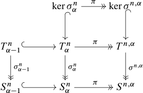
This concludes the proof.

Proposition C.2.

Assume that there exist linear maps $Δ : V \to V$ and $Γ : V \to V$ such that $Δ (V_{i}) \subseteq V_{i - 1}$ and $Γ (V_{i}) \subseteq V_{i}$ for every $i \in ℕ$ and such that $[Δ, Γ] = Δ .$ The extension of $Δ$ as a derivation of $T (V),$ respectively $S (V),$ verifies $Δ (T_{α}^{n}) \subseteq Δ (T_{α - 1}^{n}),$ respectively $Δ (S_{α}^{n}) \subseteq Δ (S_{α - 1}^{n}) .$ The extension of $Γ$ as a derivation of $T (V),$ respectively $S (V),$ stabilizes the preceding filtration on $T (V),$ respectively $S (V) .$ Hence $Δ$ and $Γ$ induce graded derivations $\bar{Δ}$ of degree $- 1$ and $\bar{Γ}$ of degree $0$ on $T (gr (V))$ and $S (gr (V)) .$ Moreover, we have $[\bar{Δ}, \bar{Γ}] = \bar{Δ} .$

In addition, $Δ$ induces a degree $- 1$ map on $gr (V),$ and $Γ$ induces a degree $0$ map on $gr (V),$ and their extensions as derivations on $T (gr (V))$ and $S (gr (V))$ coincide with $\bar{Δ}$ and $\bar{Γ} .$

Proof.

The extension of a linear map

f : V \to V

as a derivation of

T (V)

acts on

V_{α_{1}} \otimes \dots \otimes V_{α_{n}}

as

f \otimes id \otimes \dots \otimes id + \dots + id \otimes \dots \otimes id \otimes f .

Hence if

f = Δ,

then

T_{α}^{n}

is mapped into

T_{α - 1}^{n},

and if

f = Γ,

then

T_{α}^{n}

is mapped into

T_{α}^{n},

showing that they induce graded endomorphisms

\bar{Δ}

of degree

- 1

and

\bar{Γ}

of degree

0

of

T (gr (V))

and

S (gr (V)) .

Moreover, these endomorphisms are derivations of the associated graded rings and verify

[\bar{Δ}, \bar{Γ}] = \bar{Δ} .

For the last part of the proof, since the maps considered are derivations of

T (gr (V))

and

S (gr (V)),

it suffices to show that they coincide on

gr (V) .

This follows readily from the following commutative diagrams.

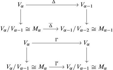
This concludes the proof.

Example C.3.

Consider

V

a finite-dimensional vector space and

Δ

and

Γ

two linear endomorphisms of

V

verifying

[Δ, Γ] = Δ .

Since

Δ

is nilpotent and

\ker Δ^{i}

is

Γ -

invariant (see the proof of Theorem 4.5), the family of subspaces

V_{i} = \ker Δ^{i}

is a filtration of

V

satisfying the hypothesis of Proposition C.2.

Acknowledgements

The authors thank Patrick Le Meur for fruitful discussions on Artin–Schelter regular algebras.

Funding

This work was partially supported by IDP and LMBP.

References

[1] J. Alev and F. Dumas, Sur le corps des fractions de certaines algèbres quantiques. J. Algebra 170 (1994), no. 1, 229–265 Zbl 0820.17015 MR 1302839
[2] M. Artin and W. F. Schelter, Graded algebras of global dimension $3$ . Adv. Math. 66 (1987), no. 2, 171–216 Zbl 0633.16001 MR 0917738
[3] J. Bell and J. J. Zhang, An isomorphism lemma for graded rings. Proc. Amer. Math. Soc. 145 (2017), no. 3, 989–994 Zbl 1400.16037 MR 3589298
[4] N. Bourbaki, Algèbre. Chapitres 1 à 3. Élém. Math., Springer, Berlin, 2007, 636 pp. Zbl 1111.00001 MR 0274237
[5] V. Coll, M. Gerstenhaber, and A. Giaquinto, An explicit deformation formula with noncommuting derivations. In Ring theory 1989. In honor of S. A. Amitsur (Proc. Sympos. Workshop, Jerusalem, Israel, 1988/89), pp. 396–403, Israel Math. Conf. Proc. 1, Weizmann, Jerusalem, 1989 Zbl 0684.16016 MR 1029329
[6] J. K. Deveney and D. R. Finston, Fields of $G_{a}$ invariants are ruled. Canad. Math. Bull. 37 (1994), no. 1, 37–41 Zbl 0804.14023 MR 1261555
[7] V. Dolgushev, The Van den Bergh duality and the modular symmetry of a Poisson variety. Selecta Math. (N.S.) 14 (2009), no. 2, 199–228 Zbl 1172.53054 MR 2480714
[8] S. Eilenberg, Homological dimension and syzygies. Ann. of Math. (2) 64 (1956), no. 2, 328–336; Errata 65 (1957), 593 Zbl 0073.26003 MR 0082489
[9] G. Freudenburg, Algebraic theory of locally nilpotent derivations. Encyclopaedia Math. Sci. 136, Springer, Berlin, 2006, 319 pp. Zbl 1121.13002 MR 2259515
[10] V. Ginzburg, Calabi–Yau algebras. [v1] 2006, [v3] 2007, arXiv:math/0612139v3
[11] K. R. Goodearl, Semiclassical limits of quantized coordinate rings. In D. Van Huynh and S. R. López-Permouth (eds.), Advances in ring theory, pp. 165–204, Trends Math., Birkhäuser, Basel, 2010 Zbl 1202.16027 MR 2664671
[12] K. R. Goodearl and S. Launois, The Dixmier–Moeglin equivalence and a Gel’fand–Kirillov problem for Poisson polynomial algebras. Bull. Soc. Math. France 139 (2011), no. 1, 1–39 Zbl 1226.17016 MR 2815026
[13] K. R. Goodearl and R. B. Warfield Jr., An introduction to noncommutative Noetherian rings, 2nd edn., London Math. Soc. Stud. Texts 61, Cambridge University Press, Cambridge, 2004, 344 pp. Zbl 1101.16001 MR 2080008
[14] C. Laurent-Gengoux, A. Pichereau, and P. Vanhaecke, Poisson structures. Grundlehren Math. Wiss. 347, Springer, Heidelberg, 2013, 464 pp. Zbl 1284.53001 MR 2906391
[15] C. Lecoutre, Polynomial Poisson algebras: Gel’fand–Kirillov problem and Poisson spectra. Ph.D. thesis, University of Kent, 2014, https://kar.kent.ac.uk/47941/ visited on 17 April 2026
[16] C. Lecoutre and S. J. Sierra, A new family of Poisson algebras and their deformations. Nagoya Math. J. 233 (2019), 32–86 Zbl 1461.16032 MR 3901632
[17] J. Luo, S.-Q. Wang, and Q.-S. Wu, Twisted Poincaré duality between Poisson homology and Poisson cohomology. J. Algebra 442 (2015), 484–505 Zbl 1392.17015 MR 3395070
[18] J. C. McConnell, Representations of solvable Lie algebras and the Gelfand–Kirillov conjecture. Proc. Lond. Math. Soc. (3) 29 (1974), no. 3, 453–484 Zbl 0323.17005 MR 0357529
[19] A. Nowicki, Polynomial derivations and their rings of constants, Uniwersytet Mikołaja Kopernika, Toruń, 1994, 170 pp. Zbl 1236.13023 MR 2553232
[20] S.-Q. Oh, Poisson polynomial rings. Comm. Algebra 34 (2006), no. 4, 1265–1277 Zbl 1135.17012 MR 2220812
[21] A. I. Ooms, The Gelfand–Kirillov conjecture for semi-direct products of Lie algebras. J. Algebra 305 (2006), no. 2, 901–911 Zbl 1169.17006 MR 2266859
[22] B. Pym, Quantum deformations of projective three-space. Adv. Math. 281 (2015), 1216–1241 Zbl 1338.14007 MR 3366864
[23] M. Reyes, D. Rogalski, and J. J. Zhang, Skew Calabi–Yau algebras and homological identities. Adv. Math. 264 (2014), 308–354 Zbl 1336.16011 MR 3250287
[24] D. Rogalski, Noncommutative projective geometry. Math. Sci. Res. Inst. Publ. 64 (2016), 13–70 Zbl 1386.14016 MR 3618472
[25] X. Tang, X. Wang, and J. J. Zhang, Twists of graded Poisson algebras and related properties. J. Geom. Phys. 207 (2025), article no. 105344, 31 pp. Zbl 1557.17027 MR 4818305
[26] P. Tauvel and R. W. T. Yu, Algèbres de Poisson et algèbres de Lie résolubles. Comm. Algebra 38 (2010), no. 6, 2317–2353 Zbl 1246.17028 MR 2675540
[27] A. van den Essen, Locally nilpotent derivations and their applications. III. J. Pure Appl. Algebra 98 (1995), no. 1, 15–23 Zbl 0821.13002 MR 1316994
[28] A. van den Essen, Polynomial automorphisms and the Jacobian conjecture. Progr. Math. 190, Birkhäuser, Basel, 2000, 329 pp. Zbl 0962.14037 MR 1790619
[29] P. Vanhaecke, Integrable systems in the realm of algebraic geometry, 2nd edn., Lecture Notes in Math. 1638, Springer, Berlin, 2001, 264 pp. Zbl 0997.37032 MR 1850713
[30] R. Vidal, Automorphismes et dérivations de “petites normes” sur un corps valué non archimédien. Ann. Sci. Univ. Clermont-Ferrand II Math. 73 (1982), no. 21, 87–95 Zbl 0536.46050 MR 0706125
[31] Q. Wu and R. Zhu, Nakayama automorphisms and modular derivations in filtered deformations. J. Algebra 572 (2021), 381–421 Zbl 1473.16006 MR 4200729

Cite this article

Vincent Beck, César Lecoutre, Rank two Artin–Schelter regular algebras from noncommuting derivations. J. Noncommut. Geom. 20 (2026), no. 4, pp. 1225–1277

DOI 10.4171/JNCG/679

Abstract

Introduction

1. A deformation formula for noncommuting derivations

Example 1.3.

2. Solvable pairs

2.1. Generalities

Lemma 2.1.

Proof.

Remark 2.2.

Proposition 2.3.

Proof.

Corollary 2.4.

Proof.

Example 2.5.

Example 2.6.

Example 2.7.

2.2. Center

Definition 2.8.

Lemma 2.9.

Proof.

Example 2.11.

Example 2.12.

Example 2.13.

2.3. Derivation and automorphism

Definition 2.14.

Lemma 2.15.

Remark 2.16.

Theorem 2.17.

Proof.

Lemma 2.18.

Proof.

2.4. A filtration on R(Δ,Γ)

Definition 2.19.

Lemma 2.20.

Proof.

Lemma 2.21.

Proof.

Proposition 2.22.

Proof.

Corollary 2.23.

Proof.

Example 2.24.

Example 2.25.

Example 2.26.

2.5. Normal elements

Lemma 2.27.

Proof.

Definition 2.28.

Lemma 2.29.

Proof.

Definition 2.30

Lemma 2.31.

Proof.

2.6. A canonical form up to localization

2.6.1. The Poisson case

Proposition 2.32.

Proof.

2.6.2. The noncommutative case

Proposition 2.33.

Proof.

2.7. Skewfield of fractions

Proposition 2.34.

Proof.

Remark 2.35.

3. The rank of A(Δ,Γ)

4. Linear solvable pairs

Proposition 4.1.

Proof.

Definition 4.2.

Remark 4.3.

Lemma 4.4.

Proof.

4.1. The case of Δ maximal

Theorem 4.5.

Proof.

Example 4.6.

4.2. Center in the linear case

Proposition 4.7.

Proof.

Corollary 4.8.

2.4. A filtration on $R_{(Δ, Γ)}$

3. The rank of $A_{(Δ, Γ)}$

4.1. The case of $Δ$ maximal

6.1.2. When $Δ$ is not necessarily maximal

6.1.3. When $Γ$ is not diagonal

7. Diagonalizable linear solvable pair: The algebra $R_{(Δ, Γ)}$

8.1. Unimodularity of $A_{(Δ, Γ)}$ in the polynomial case

8.2. Calabi–Yau property for $R_{(Δ, Γ)}$ in the generic diagonalizable case