Categorical absorption of a non-isolated singularity
Aporva Varshney
University College London, UK
Abstract
We study an example of a projective threefold with a non-isolated singularity and its derived category. The singular locus can be locally described as a line of surface nodes compounded with a threefold node at the origin. We construct a semiorthogonal decomposition where one component absorbs the singularity in the sense of Kuznetsov–Shinder, and the other components are equivalent to the derived categories of smooth projective varieties. The absorbing category is seen to be closely related to the absorbing category constructed for nodal varieties by Kuznetsov–Shinder, reflecting the geometry of the singularity. We further show that the semiorthogonal decomposition is induced by one on a geometric resolution and briefly consider the properties of the absorbing category under smoothing.
1. Introduction
Studying the bounded derived category of coherent sheaves of a variety over a field can often reveal information about the geometry of One way in which we may study the structure of is by considering how it can be broken down into smaller pieces: a semiorthogonal decomposition
is an ordered collection of full triangulated subcategories generating such that ‘there are no morphisms from right to left’. Precisely, for and with
Recently, there has been interest in studying when is a singular variety. One approach we may take is to consider the full triangulated subcategory of perfect complexes, that is, the complexes quasi-isomorphic to a bounded complex of locally free sheaves. When is smooth, coincides with since in this setting all coherent sheaves have a finite resolution by locally free sheaves, and so we can think of as capturing smoothness. It then makes sense to define the singularity category [19
D. O. Orlov, Triangulated categories of singularities and D-branes in Landau–Ginzburg models (in Russian). Tr. Mat. Inst. Steklova 246 (2004), 240–262. English translation. Proc. Steklov Inst. Math. 246 (2004), 227–248 Zbl 1101.81093 MR 2101296
]This category exhibits locality in the sense that it depends only on an open neighbourhood of the singular locus.
On the other hand, one can take a more global approach to studying the singularity. Suppose is a projective variety with a single isolated singularity. Then, one can consider whether the singularity is captured at the level of the derived category by asking if there exists a semiorthogonal decomposition
where so that is, in some sense, responsible for the singularity. Following [15
A. Kuznetsov and E. Shinder, Categorical absorptions of singularities and degenerations. Épijournal Géom. Algébrique (2024), article no. 12, 42 pp., (Special volume in honour of Claire Voisin) Zbl 1545.14026 MR 4698898
], we say that provides a categorical absorption of singularities. We can motivate this further as follows: there does not exist a semiorthogonal decomposition of the formbut we can try to approximate it by asking that is as large as possible. Examples studied in the literature also have the property that is equivalent to for some dg-algebra with finite-dimensional cohomology.
The existence of a categorical absorption depends not only on the singularity but also on the global structure of the variety; indeed, there are several obstructions as a result of this. Nevertheless, we briefly review several instances where such a semiorthogonal decomposition has been found. For the rest of the section, we work over
In [8
J. Karmazyn, A. Kuznetsov, and E. Shinder, Derived categories of singular surfaces. J. Eur. Math. Soc. (JEMS) 24 (2022), no. 2, 461–526 Zbl 1493.14023 MR 4382477
], the authors study surfaces with cyclic quotient singularities. These include the singularities of the weighted projective space which are shown to have a semiorthogonal decompositionwhere For surfaces with type singularities, it is shown that the singularity is often absorbed by the algebra with with a simple example being the blow-up of a smooth surface in a non-reduced point A semiorthogonal decomposition is produced for the threefold in [9
Y. Kawamata, On the derived category of a weighted projective threefold. Boll. Unione Mat. Ital. 15 (2022), no. 1–2, 245–252 Zbl 1492.14028 MR 4390551
]:where this time is an algebra with
The most relevant case for us will be categorical absorption of nodal varieties. Nodal threefolds are considered in various incarnations in [10
Y. Kawamata, Semi-orthogonal decomposition of a derived category of a 3-fold with an ordinary double point. In H. Abban, G. Brown, A. Kasprzyk, and S. Mori (eds.), Recent developments in algebraic geometry. To Miles Reid for his 70th birthday, pp. 183–215, London Math. Soc. Lecture Note Ser. 478, Cambridge University Press, Cambridge, 2022 Zbl 1524.14040 MR 4480569
, 21N. Pavic and E. Shinder, Derived categories of nodal del Pezzo threefolds. Taiwanese J. Math. 29 (2025), no. 6, 1607–1632 Zbl 08150207 MR 5003266
, 22F. Xie, Nodal quintic del Pezzo threefolds and their derived categories. Math. Z. 304 (2023), no. 3, article no. 48, 28 pp. Zbl 1528.14022 MR 4610379
]. We follow the approach detailed in [15A. Kuznetsov and E. Shinder, Categorical absorptions of singularities and degenerations. Épijournal Géom. Algébrique (2024), article no. 12, 42 pp., (Special volume in honour of Claire Voisin) Zbl 1545.14026 MR 4698898
]. To illustrate this theory, let be a nodal genus curve consisting of curves intersecting transversely at a point. The contraction of the branch through the map yields the semiorthogonal decompositionwhere we have that is fully faithful. Absorption is then given by the category and denoting one finds that
where and We say that is a object, since resembles the cohomology ring of It was shown in [15
A. Kuznetsov and E. Shinder, Categorical absorptions of singularities and degenerations. Épijournal Géom. Algébrique (2024), article no. 12, 42 pp., (Special volume in honour of Claire Voisin) Zbl 1545.14026 MR 4698898
] that objects can be used to absorb singularities on nodal varieties of odd dimension. In contrast, in even dimensions, the absorbing category is instead given by with and with In this case, is called a object.Perhaps the most interesting part of this story is a property of objects known as deformation absorption: given a object on a variety, the pushforward into a smoothing of the variety generates an admissible subcategory of the smoothing. Essentially, this tells us that the object vanishes from the semiorthogonal decomposition when smoothing the variety. In the example above, this is exemplified by considering a smoothing of to This powerful property was used in [16
A. Kuznetsov and E. Shinder, Derived categories of Fano threefolds and degenerations. Invent. Math. 239 (2025), no. 2, 377–430 Zbl 1564.14091 MR 4850600
] to study relationships between the Kuznetsov components of smooth Fano threefolds, by first degenerating a threefold to a nodal variety and then taking a resolution.1.1. Results and structure
The cases in the literature have so far focused on isolated singularities. Presently, we turn our attention to a complex threefold with a non-isolated compound singularity, constructed as follows. We first consider the curve
and then perform a blow-up
Then, is locally given by the equation so we can think of the singularity as a family of surface nodes compounded with a threefold node at the origin. In this article, we essentially perform a series of calculations, checking that there is a categorical absorption which is as nicely behaved as one could expect.
Theorem 1.1
( Theorem 3.3). The curve and threefold admit a categorical absorption, where the absorbing category is generated by an object with the property
where and
We call an object with this self-Ext algebra a compound or object, to reflect the idea that it is simultaneously a and object.
The work in [16
A. Kuznetsov and E. Shinder, Derived categories of Fano threefolds and degenerations. Invent. Math. 239 (2025), no. 2, 377–430 Zbl 1564.14091 MR 4850600
] shows us that it can be useful to consider the structure of a resolution and of a smoothing; consequently, in Section 4, we show that the semiorthogonal decomposition produced for is induced by one on a specific choice of resolution of singularities In particular, our resolution has as an exceptional divisor a surface and a curve intersecting transversely. The key geometric input which allows us to perform computations in the derived category of is the following proposition.Proposition 1.2
( Proposition 4.3). The space can be obtained from as a series of blow-ups along smooth rational curves.
Using this, we obtain a full exceptional collection on However, this collection is not compatible with the contraction in the sense that the pushforward under does not recover the absorption constructed on To overcome this, we perform a series of mutations and explicitly find an admissible category that serves as a ‘categorical resolution’ for our absorbing category.
Theorem 1.3
( Theorem 4.8). Let be the resolution of singularities map. There is an admissible subcategory such that the absorbing category is equivalent to the Verdier quotient
The category is generated by an exceptional collection of length and under the pushforward all the generating objects are mapped to the object We investigate the algebra structure of this collection.
Theorem 1.4
( Theorem 4.16). The morphisms in the exceptional sequence
are described as follows:
- (1)
- (2)
- (3)
- (4)
To compute how morphisms compose, we note that there is an isomorphism of graded vector spaces between the spaces in the theorem above and the truncated self-Ext-spaces of the object:
This indicates that the morphisms between objects of should be seen as lifting some map We prove the following.
Proposition 1.5
( Proposition 4.19). All compositions in are non-zero.
In particular, omitting compositions in non-zero degrees, we can visualise the categorical resolution as the following quiver.
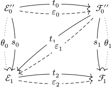
Here, solid arrows indicate degree maps, dashed arrows indicate degree maps and dotted arrows indicate degree maps.
Finally, we briefly consider the properties of our objects with respect to smoothings of the curve in Section 5.
Proposition 1.6
( Proposition 5.1). Let be the smoothing of obtained by blowing up in a fattened point Then, the pushforward of the object into generates an admissible subcategory of and hence provides a deformation absorption with respect to the smoothing
Notation and conventions.
- (1)We work over the base field
- (2)For a dg-algebra with finite-dimensional cohomology, we denote by the unbounded derived category of dg-modules over and is the subcategory of dg-modules with finite-dimensional total cohomology.
- (3)Tensor products and pushforward and pullback functors between derived categories are implicitly derived.
- (4)Given a scheme with closed subscheme and a birational map we denote by the strict transform of in
2. Preliminaries
2.1. Derived categories
In this section, we recap general results in the theory of derived categories which we will use freely.
2.1.1. Mutations of semiorthogonal decompositions. Given a semiorthogonal decomposition of a triangulated category where each component is admissible
it is possible to reorder the components to obtain a new semiorthogonal decomposition. The first method is to perform a left mutation of over
and the second is to perform a right mutation of over
In each case, the mutation is an equivalence of categories
We omit the construction, but note that when and are generated by exceptional objects and respectively, we have formulae for the left and right mutations through the following exact triangles [4
A. I. Bondal, Representation of associative algebras and coherent sheaves (in Russian). Izv. Akad. Nauk SSSR Ser. Mat. 53 (1989), no. 1, 25–44. English translation. Math. USSR-Izv. 34 (1990), no. 1, 23–42 Zbl 0692.18002 MR 0992977
]:We also note an easy consequence of Serre duality.
Lemma 2.1.
If is Gorenstein with a semiorthogonal decomposition
we have that
is also a semiorthogonal decomposition, where is the canonical bundle.
2.1.2. Derived nine-lemma. When working in the derived category, the ordinary nine-lemma in homological algebra no longer holds. Instead, we have the following derived nine-lemma (see [17
J. P. May, The additivity of traces in triangulated categories. Adv. Math. 163 (2001), no. 1, 34–73 Zbl 1007.18012 MR 1867203
, Lemma 2.6] for a proof).Lemma 2.2.
Suppose that the top-left square commutes in the following diagram and the top two rows and left two columns are exact triangles.
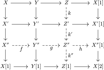
Then, there exists an object and maps such that the bottom-right square anti-commutes, all other squares commute and all rows and columns form exact triangles.
2.1.3. Derived category of a blow-up. Suppose is a scheme and is a locally complete intersection of codimension Consider the blow-up Then, there is a semiorthogonal decomposition [18
D. O. Orlov, Projective bundles, monoidal transformations, and derived categories of coherent sheaves (in Russian). Izv. Ross. Akad. Nauk Ser. Mat. 56 (1992), no. 4, 852–862. English translation. Russ. Acad. Sci. Izv. Math. 41 (1993), no. 1, 133–141 Zbl 0798.14007 MR 1208153
]where is embedded fully faithfully by pulling back, and the functors are fully faithful and constructed as follows. The exceptional divisor is a projective bundle over so letting be the inclusion, we define
2.1.4. The cone on the pull-push counit. Let be the inclusion of a Cartier divisor in a scheme A useful computation tool will be the following description of the cone on the canonical adjunction morphism [2
A. Bondal and D. Orlov, Semiorthogonal decomposition for algebraic varieties. 1995 arXiv:alg-geom/9506012v1
]:2.1.5. Bondal–Orlov localisation. The Bondal–Orlov localisation conjecture relates the derived categories of a singular variety and a resolution
Conjecture 2.3
([6
A. I. Efimov, Homotopy finiteness of some DG categories from algebraic geometry. J. Eur. Math. Soc. (JEMS) 22 (2020), no. 9, 2879–2942 Zbl 1478.14010 MR 4127943
, Conjecture 1.9], [3A. Bondal and D. Orlov, Derived categories of coherent sheaves. In Proceedings of the International Congress of Mathematicians, Vol. II (Beijing, 2002), pp. 47–56, Higher Ed. Press, Beijing, 2002 Zbl 0996.18007 MR 1957019
, Section 5]). If is a resolution of rational singularities, then induces an equivalence between and a Verdier quotient of :In fact, the conjecture is true in several settings (see [6
A. I. Efimov, Homotopy finiteness of some DG categories from algebraic geometry. J. Eur. Math. Soc. (JEMS) 22 (2020), no. 9, 2879–2942 Zbl 1478.14010 MR 4127943
, 20N. Pavic and E. Shinder, theory and the singularity category of quotient singularities. Ann. K-Theory 6 (2021), no. 3, 381–424 Zbl 1490.14020 MR 4310324
]). The most relevant situation for us will be when the resolution has one-dimensional fibres, in which case the conjecture was proven in [1A. Bondal, M. Kapranov, and V. Schechtman, Perverse schobers and birational geometry. Selecta Math. (N.S.) 24 (2018), no. 1, 85–143 Zbl 1436.14037 MR 3769727
]. An immediate consequence of this is that we may descend an appropriate semiorthogonal decomposition of to one for [15A. Kuznetsov and E. Shinder, Categorical absorptions of singularities and degenerations. Épijournal Géom. Algébrique (2024), article no. 12, 42 pp., (Special volume in honour of Claire Voisin) Zbl 1545.14026 MR 4698898
, Proposition 4.1]. Ifis a semiorthogonal decomposition such that then we obtain a semiorthogonal decomposition
with
where must generate because is essentially surjective.
2.1.6. Spherical objects. An object where is a complex smooth and projective variety, is called spherical if [7
D. Huybrechts, Fourier–Mukai transforms in algebraic geometry. Oxford Math. Monogr., Oxford University Press, Oxford, 2006, 307 pp. Zbl 1095.14002 MR 2244106
]- (1)and
- (2)
where is the sphere of dimension equal to A spherical object induces an autoequivalence of the derived category by twisting around the object. For any object the twist is defined through the exact triangle
Being an autoequivalence, it has an inverse known as the dual twist, which is similarly described by an exact triangle.
2.2. Projective bundles and ruled surfaces
We review some theory which will be essential for computations later on. Fix a smooth variety and let and be invertible sheaves. Let Then, there are two possible conventions for the corresponding projective bundle; in our case, we take the definition to be
so that there is a map We will write to denote that the coordinates on the fibres are There is a section corresponding to the surjection equivalently, it is given by the vanishing of the coordinate The skyscraper sheaf of the section is defined by taking the cokernel of the composition yielding
and twisting by
Then, the above sequence is the Koszul resolution of so it follows from the fact that that the normal bundle of is given by Note that the first map is ‘multiplication by ’, and hence is a section of the line bundle
We collect some results on ruled surfaces, which will arise frequently when we blow up a curve in a smooth threefold In this situation, we recall that the exceptional divisor is isomorphic to and has normal bundle Consider
Then, the divisor corresponding to is given by the class of the section and we denote
or, equivalently, it is the line bundle corresponding to the divisor where is a fibre. Then, the canonical bundle is given by the formula
If then pushing forward the line bundle to the base gives us
2.3. Categorical absorption for nodal varieties
This section gives an overview of the theory of categorical absorption for nodal varieties, with [15
A. Kuznetsov and E. Shinder, Categorical absorptions of singularities and degenerations. Épijournal Géom. Algébrique (2024), article no. 12, 42 pp., (Special volume in honour of Claire Voisin) Zbl 1545.14026 MR 4698898
] as our primary reference. We will only concern ourselves with dimensions up to but note that the theory can be extended to arbitrary dimension.2.3.1. Categorical ordinary double points. We recall the definitions given earlier.
Definition 2.4.
An object for a variety is called a object if
Definition 2.5.
The categorical ordinary double point of degree is with
The theory is split up by parity of : in all examples, when is even dimensional, and when is odd dimensional.
For the odd-dimensional case, the key example is the nodal curve considered earlier, which we can see as the vanishing locus
In this case, the pushforward of a line bundle on either of the two branches gives a object. We have seen that we can consider contracting one of the branches it is then a direct consequence of the fact that that the pullback is fully faithful. One can show that the null category is admissible in this case, and that there is a semiorthogonal decomposition [15
A. Kuznetsov and E. Shinder, Categorical absorptions of singularities and degenerations. Épijournal Géom. Algébrique (2024), article no. 12, 42 pp., (Special volume in honour of Claire Voisin) Zbl 1545.14026 MR 4698898
, Proposition 6.15]with Here, the absorbing category is generated by the pushforward of the sheaf on the branch being contracted.
The simplest (but still useful) example of a nodal even-dimensional scheme is the fat point In this case, the object is a object which generates where More interestingly, we may consider the nodal surface [8
J. Karmazyn, A. Kuznetsov, and E. Shinder, Derived categories of singular surfaces. J. Eur. Math. Soc. (JEMS) 24 (2022), no. 2, 461–526 Zbl 1493.14023 MR 4382477
, Example 3.17]. To construct a categorical absorption here, we consider the resolution of singularities given bywhere we denote by the second Hirzebruch surface. In this case, the exceptional divisor is given by the section of the bundle which has self-intersection and it can be shown that the kernel of is generated by Let be the class of a fibre, so that Then, is the divisor corresponding to and so there is a full exceptional sequence
One sees that there is a short exact sequence
which implies that An important feature here is that the sheaf is a spherical object, and is the dual spherical twist of around We note that the pushforwards and remain exceptional in and hence is a candidate for our categorical absorption. We can compute, using (2.6), that
Since the cone on the morphism is in we find that
The idea is that this object should be a object; intuitively, the degree 0 morphism becomes an isomorphism and the degree morphism then gives rise to the self-extension of the object.
These observations are formalised in the following theorems.
Definition 2.6
([15
A. Kuznetsov and E. Shinder, Categorical absorptions of singularities and degenerations. Épijournal Géom. Algébrique (2024), article no. 12, 42 pp., (Special volume in honour of Claire Voisin) Zbl 1545.14026 MR 4698898
, Section 3.1]). The graded Kronecker quiver of degree is the path dg-algebra of the following dg-quiver: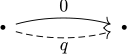
where there are two arrows of degrees and respectively, and the differentials are zero. The graded Kronecker quiver category of degree denoted is the derived category of this algebra.
Theorem 2.7
([15
A. Kuznetsov and E. Shinder, Categorical absorptions of singularities and degenerations. Épijournal Géom. Algébrique (2024), article no. 12, 42 pp., (Special volume in honour of Claire Voisin) Zbl 1545.14026 MR 4698898
, Corollary 3.3]). Let be an exceptional sequence, where is a variety such that Then, Theorem 2.8
([15
A. Kuznetsov and E. Shinder, Categorical absorptions of singularities and degenerations. Épijournal Géom. Algébrique (2024), article no. 12, 42 pp., (Special volume in honour of Claire Voisin) Zbl 1545.14026 MR 4698898
, Proposition 3.7]). Let and define the object using the distinguished triangleThen, is a spherical object, and there is an equivalence
and the image of under is a object.
In the more general setting, the theorem can be applied as follows. Suppose we have a crepant resolution for a nodal surface or threefold and assume that we have so that line bundles are exceptional objects. Then, labeling the exceptional curve as we have a spherical object where One can show that generates Now suppose is an exceptional object such that A simple way to find such an object is to look for a divisor which intersects the curve transversely at a point, and then take the associated line bundle. Now, we can simply take the spherical twist of around if is concentrated in degree this takes the form
Since a spherical twist is an autoequivalence, we see that is an exceptional object, so we have an admissible subcategory of which contains It is then not hard to show, simply by taking long exact sequences for that for and hence taking the Verdier quotient gives us a object generating a categorical ordinary double point of degree As a result, we are able to construct a categorical absorption for the nodal variety.
2.3.2. Deformation absorption. Finally, we discuss smoothings of nodal varieties. Suppose that is a flat projective morphism from a smooth space to a smooth curve with the central fibre isomorphic to and all other fibres smooth, so that gives a smoothing of Now suppose that the nodal variety has an absorption by a object as follows:
Then, for any smoothing the object can be shown to be exceptional [15
A. Kuznetsov and E. Shinder, Categorical absorptions of singularities and degenerations. Épijournal Géom. Algébrique (2024), article no. 12, 42 pp., (Special volume in honour of Claire Voisin) Zbl 1545.14026 MR 4698898
, Theorem 1.8]. In particular, we have a semiorthogonal decompositionwhich is said to be linear in the sense that there is a well-defined notion of base changing the semiorthogonal decomposition to a fibre of the map [13
A. Kuznetsov, Base change for semiorthogonal decompositions. Compos. Math. 147 (2011), no. 3, 852–876 Zbl 1218.18009 MR 2801403
]. Performing this base change to a non-central fibre we find that the component vanishes since it is only supported on the central fibre, and soIn effect, we have a family of smooth and proper categories and for we acquire a object to account for the singular behaviour. We say that objects provide a deformation absorption, and furthermore, since this occurs for every smoothing, we say that the deformation absorption is universal.
3. Compound objects
We begin by generalising the example of a nodal curve by trivially thickening one of the branches. Consider
which is a copy of intersecting the thickened branch
at a fat point. There is a contraction and it follows once again from the fact that that there is a semiorthogonal decomposition
with fully faithful. Let be the reduction of the fattened branch Denote by the pushforward of the line bundle on to
Lemma 3.1.
The kernel of is generated by
Proof.
Firstly, consider the projections and Then, we have that
where we denote by the generator of The pushforward of this sheaf to is precisely
To reduce to this case, we show that any object in the kernel of is a pushforward of an object in Firstly, let be a sheaf on supported set-theoretically on Then, we can find a short exact sequence
where is contained in for some and Now assume that is a thickening of so that and hence Since we find that Now, left exactness of implies that Hence, any sheaf has scheme-theoretic support contained in
Finally, if is a complex, we use a standard spectral sequence argument (see, e.g., [5
T. Bridgeland, Flops and derived categories. Invent. Math. 147 (2002), no. 3, 613–632 Zbl 1085.14017 MR 1893007
, Lemma 3.1]) usingThis degenerates on the second page, so that if is a thickening of then the non-vanishing of for some implies the non-vanishing of
Now we let denote the restriction of the line bundle on with degree along and degree along Then, the object has an infinite locally free resolution
so that can be computed using the chain complex
where all maps are zero, since the coordinate becomes when restricted to Hence, is the pushforward of a line bundle on and to compute global we can simply take global sections as the local-to-global spectral sequence degenerates on the second page. If is even, then this shows that has dimension with basis given by If is odd, then has dimension with basis given by Concretely, the dimensions of form a sequence: We guess from this observation that the algebra structure is that of a polynomial ring with a generator of degree and a generator of degree this guess is verified in the next theorem.
Definition 3.2.
An object for a variety is called a compound object, or if there is an isomorphism of graded algebras
where and
Theorem 3.3.
The object is a object on
Proof.
Consider the locally free resolution for The element of arises from the mapping
and we lift this to a morphism by defining a chain map on the locally free resolution, so that all triangles and quadrilaterals in the diagram below commute.

Next, has a basis given by the elements We lift the element given by to a chain map similarly.

One now sees that since both compositions are given by the chain map lifting the element

In general, we claim that the lift of the element is given by the chain map if is even, and if is odd. This is verified by observing that in the even case, the chain map lifting is given by
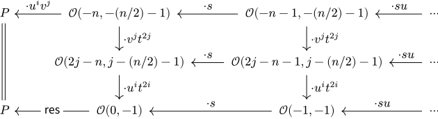
while in the odd case, the chain map lifting is given by
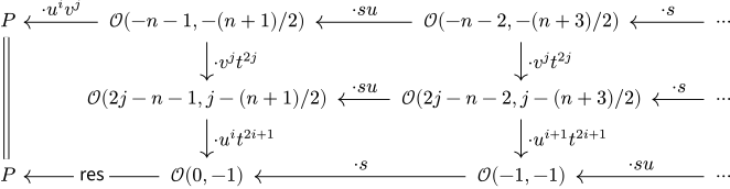
hence concluding the proof.
Remark 3.4.
In fact, the above proof shows that the algebra is formal, that is, quasi-isomorphic to The chain maps constructed above give us the quasi-isomorphism.
Remark 3.5.
There is in fact a general class of examples where one can perform the same trick, given by considering the trivially thickened curve intersecting a smooth curve transversely. For with defined analogously, the algebra will not be formal.
Note that Hence, by the Serre duality statement of Lemma 2.1, we also have the following semiorthogonal decomposition for which we will use in the sequel.
Note here that is the skyscraper sheaf along and we will define
to be the absorbing subcategory of
Remark 3.6.
Given a object we expect that there is an equivalence given by Koszul duality
This would follow by computing over the algebra After verifying that the dg-algebras involved are formal, for example, using a similar argument to the one given in Remark 3.4, the desired Koszul duality statement would then follow from [11
B. Keller, Derived categories and tilting. In L. A. Hügel, D. Happel, and H. Krause (eds.), Handbook of tilting theory, pp. 49–104, London Math. Soc. Lecture Note Ser. 332, Cambridge University Press, Cambridge, 2007 MR 2384608
, Theorem 8.5 (b)].4. Semiorthogonal decomposition for a resolution of singularities
Let be a smooth threefold which contains the curve considered in Section 3 as a locally complete intersection. In this section, to allow us to perform explicit calculations, we will also assume that contains an open subset
such that is just the curve missing a point at infinity on the reduced branch. For example, we may take
which contains as the vanishing locus and as the locus Let be the threefold constructed through the blow-up
Then, is singular with a line of surface nodes compounded with a threefold nodal singularity at one point. In particular, this singularity is non-isolated. By Orlov’s blow-up formula given in equation (2.1) combined with the absorption for given by equation (3.2), we immediately obtain a semiorthogonal decomposition
where is the absorbing category as in (3.3), generated by the object
It is worth considering how each component of the decomposition is embedded, using (2.2). Firstly, we define a line bundle on
which is the pullback of a line bundle via the contraction map Note has degree along the branch and is trivial along the thickened branch.
Next, is embedded into by the functor which pulls back to the exceptional locus, tensors with the bundle and pushes forward into Since is the blow-up of along we observe that the exceptional locus has two components, both of which are bundles:
We can also pullback along to obtain
Then, we can write our semiorthogonal decomposition as
where the sheaves are supported on and is supported on Note that we have chosen
Locally over takes the form
and hence has a compound singularity of the form described previously. We find that our semiorthogonal decomposition provides a categorical absorption for this singularity. The goal of this section is to show that the semiorthogonal decomposition descends from one for a resolution of
Remark 4.1.
If we instead start with intersecting a transversely, then we obtain a threefold with a non-isolated compound singularity locally given by the equation
so that we have a line of surface singularities, compounded with a threefold node at the origin.
4.1. Constructing a geometric resolution
We now describe the process of constructing the resolution, and refer to Figure 1 for a visualisation. To resolve the singularities, we first blow up along the exceptional component defined in (4.2) to obtain a singular threefold and the map
Since intersects the singular locus only at the threefold node, we find that has a family of surface node singularities. To resolve these, we blow up along the strict transform of defined in (4.3) to obtain a smooth threefold and the map
Define
to be the composition
It may be helpful to refer to the surface analogue: we may consider the blow-up
so that the exceptional divisor is a thickened and the space has a nodal singularity at the point Then, blowing up the reduced exceptional divisor gives a minimal resolution of the singularity; our second blow-up is a family version of this process.
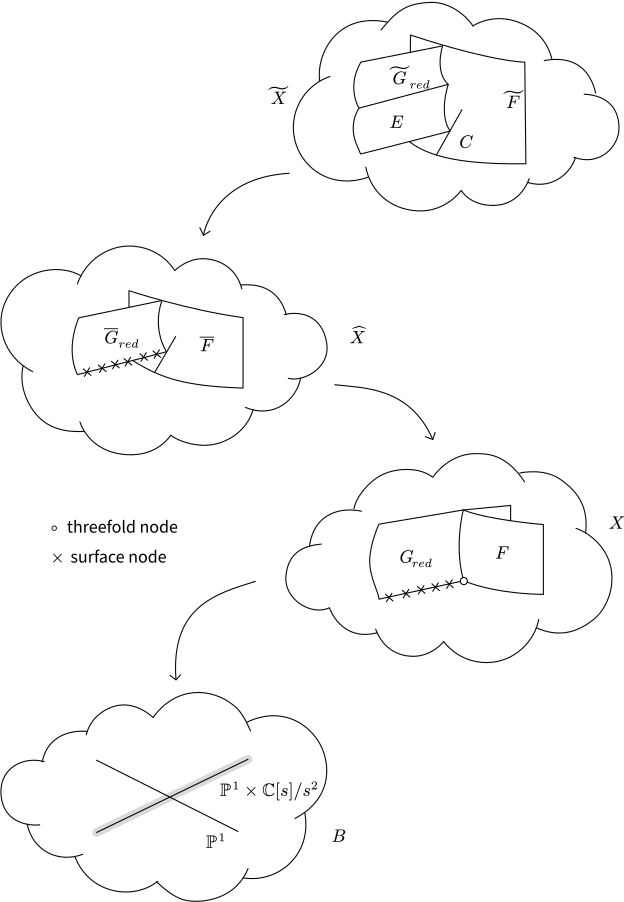
Constructing the resolution. Here, denote the strict transforms in and denote the strict transforms in
4.1.1. Local analysis. We illustrate this construction locally by considering the open subset defined in (4.1). Recall that we obtain an open subset of
Locally, and To obtain an open subset of we blow up at the ideal to obtain
where we denote We can now resolve the singularities by blowing up at :
where this time we are denoting and is the tautological line bundle on As a GIT quotient, is constructed as the quotient with weights shown in Table 1.
Matrix of weights for with omitted values equal to
Note that the exceptional locus of is a curve We denote by
the strict transform of this curve in The strict transform of in intersects the singular locus along the section where the fibre coordinate vanishes. The effect of blowing up this locus is to introduce an exceptional surface The exceptional locus of the composition is the union and it is precisely the preimage of the reduced singular locus Note that the two subvarieties and intersect transversely at a point.
Lemma 4.2.
Let be the strict transform of in Then, we have
Proof.
In the locus is given by and so its strict transform is given by The second statement follows from similarly noting that
We also see that the strict transform of intersected with is a nodal surface
which is isomorphic to the blow-up of at a fattened point cut out by the ideal Denoting by the strict transform of in we find that is a ruled surface blown up at a point, and then blown up again at a point on the exceptional curve.
4.1.2. Alternative construction of the resolution. A key computational tool will be the following alternative construction of where we only blow up smooth varieties along a This allows us to easily obtain a concrete semiorthogonal decomposition for
Proposition 4.3.
There are varieties and a sequence of contractions where each map is a blow-up of a smooth rational curve such that the following diagram commutes.
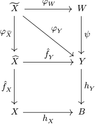
Furthermore, letting be the exceptional loci of respectively, and the strict transforms of respectively, to we have that
- (1)coincides with
- (2)coincides with
- (3)coincides with
Proof.
The map is obtained by blowing up along the reduced branch
to obtain a variety Now, can be obtained by blowing up the strict transform of the non-reduced branch Hence, we have a map and we see that the total transform of the ideal cutting out the reduced curve is locally principal in Letting be the blow-up in we see that factors as by the universal property of blow-ups.
Note that outside of the open subset both constructions of only blow up at the single point at infinity on otherwise, all blow-ups have centres contained in some open set over Define an open subset of over as
Similarly, there is an open subset of found by blowing up at and pulling back, giving
where we denote Finally, we blow up along the ideal and pull back the equations for to give
where we denote It is clear that (e.g., by writing out the matrix of weights for and comparing with Table 1), and so we recover
The centre of is given by and the exceptional locus of is given by
The centre of the blow-up is given by which is a copy of arising as a section of and we see that
is the exceptional divisor of the blow-up Now, it is clear by considering the equations cutting out each subvariety that coincides with and coincides with in It is also clear that coincides with in since both give the preimage of along the map
The alternative construction is visualised in Figure 2.
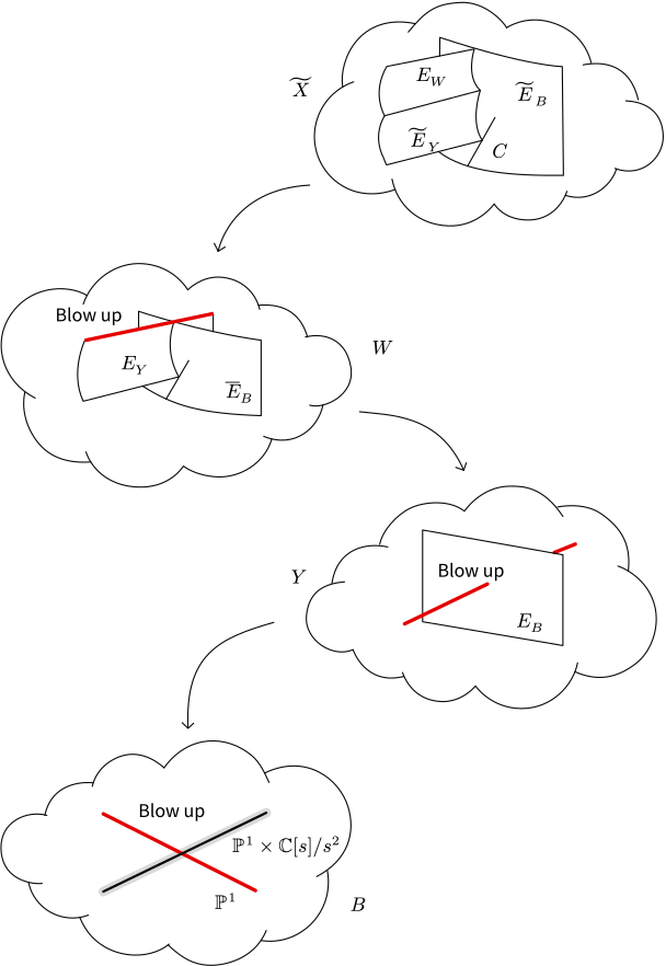
Alternative construction of the resolution, with blow-up centres indicated in red. Here, denotes the strict transform of to and denote the strict transforms of respectively, to
4.1.3. Exceptional loci. Next, we consider the irreducible component of the exceptional locus of recalling the notation for line bundles on a ruled surface introduced in equation (2.4).
Lemma 4.4.
For the divisor we have that
Proof.
Recall that by Lemma 4.2. The bundle has degree along the fibres of the bundle which we can see by considering that each fibre is the exceptional curve in the resolution of a surface node. Also note that since is the strict transform of is the blow-up of along the section given by This implies that the restriction of to the section is the same as the restriction of to Hence, we find that and using the formula for given in (2.5), we compute that
Finally, we consider the curve Recall the definition of a spherical object from Section 2.1.6.
Lemma 4.5.
The object is a spherical object in
Proof.
This follows if we can contract to an ordinary double point. Starting from let be the union of the reduction of the branches, and consider the blow-up
so that is a nodal variety. Now note that the total transform of the locus in is the union of which is a Cartier divisor, and the centre of the blow-up It follows from the universal property of the blow-up that can be written as a blow-up of at the strict transform of which is a ruled surface in intersecting the node. In particular, there is an exceptional curve which contracts to give the node. The blow-up has centre disjoint from and we can compute by working locally over that is identified with the curve under the blow-up. Hence, can also be contracted to a threefold node.
4.2. A full exceptional sequence on the resolution
With the geometric setup established, we may now analyse using Orlov’s blow-up formula once again. We recall the exceptional loci in the alternative construction from Section 4.1.3, as well as the maps described in diagram (4.5). The centre of each blow-up in the alternative construction is a locally complete intersection. This gives us the following semiorthogonal decompositions, where for a bundle embedded into a variety as we denote by the pushforward :
The component in the semiorthogonal decomposition equivalent to is immediately seen to be orthogonal to We therefore consider the following objects:
so that lies in the exceptional sequence
It is useful to obtain a geometric description for the objects and The following lemmas are certainly specialisations of more general results on the properties of pulling back skyscraper sheaves along blow-ups, but we give the concrete calculations here for completeness, using the properties of ruled surfaces given in Section 2.2.
Lemma 4.6.
For is the pushforward of the line bundle on which is
- (1)the line bundle on
- (2)the line bundle on
Proof.
We show the statement for using its description from equation (4.6), and the corresponding statement for follows by twisting appropriately. Firstly, taking the exact sequence on
and applying the pullback shows that we have an exact sequence
on Note that this statement holds even though the functor is derived; in other words, vanishes for We find that the objects are supported on Note that and is a section of Hence,
and since where is a section of we have
We hence find that is a pushforward of the line bundle on which is given by on the component and on the component. Note that the line bundle on restricts to on so such a line bundle exists on
Recall that by Proposition 4.3, coincides with the strict transform of in
Lemma 4.7.
For the objects are given as
Proof.
For the object we have a short exact sequence
so that is the pushforward of the normal bundle of Recall that is a ruled surface blown up twice, and has a chain of exceptional curves where we denote and We denote by where is the blow-up map. Then, the normal bundle must be of the form
We know that and since and the restriction to the fibres of is generically unchanged. Next, one computes via the inclusion that Since we find that
Similarly, and so we find that
Hence, and we obtain the statement for with the case of being similar.
Observe now that naïvely pushing down this semiorthogonal decomposition via does not recover the semiorthogonal decomposition we have for Recall that we expressed our semiorthogonal decomposition as
where is the embedding induced by Orlov’s blow-up formula. We recall that denotes the line bundle on which has degree over the reduced branch and is trivial over the non-reduced branch, and is the absorbing category. We can see that while Hence, we immediately see that is our object but is a different object, namely Meanwhile, the objects are supported on and hence push down to sheaves supported only on
It turns out that we can obtain a suitable exceptional sequence which recovers the semiorthogonal decomposition after pushing down simply by mutating the existing sequence appropriately.
Firstly, starting with the exceptional sequence
we find that the objects are orthogonal in Section 4.3.2, so that
is also an exceptional sequence. Then, we perform a series of left and right mutations, using the distinguished triangles described in Section 2.1.1.
Theorem 4.8.
Let
Then, there is a semiorthogonal decomposition of given by
such that:
- (1)and
- (2)the admissible subcategory defined using the exceptional sequenceinduces an equivalencewhere is the absorbing category.
The mutations performed in the above theorem are as follows:
where we firstly mutate to the left of and then mutate to the right of The theorem then states that pushforward under recovers the semiorthogonal decomposition of In particular, once the image of each component under is identified, the final statement follows as a consequence of Bondal–Orlov localisation, as described in Section 2.1.5. Since is an admissible component of a smooth projective variety, we suggest thinking of it as a categorical resolution for the absorbing category. Note that there are various formalisations of the notion of a categorical resolution in the literature (see, e.g., [12
A. Kuznetsov, Lefschetz decompositions and categorical resolutions of singularities. Selecta Math. (N.S.) 13 (2008), no. 4, 661–696 Zbl 1156.18006 MR 2403307
, 14A. Kuznetsov and V. A. Lunts, Categorical resolutions of irrational singularities. Int. Math. Res. Not. IMRN 2015 (2015), no. 13, 4536–4625 Zbl 1338.14020 MR 3439086
]); here, we use the term less formally.In the following Sections 4.3 and 4.4, we firstly obtain a complete description of the morphisms in the original exceptional sequence (4.7), as well the morphisms between the exceptional objects and to the objects in Using this, we are then able to perform the necessary mutations, and give a proof of Theorem 4.8.
4.3. Morphisms in the exceptional sequence
4.3.1. Morphisms to the null category. We firstly compute the morphisms between each object in the collection and some key objects in the kernel. The results are summarised in Tables 2 and 3.
| 0 | 0 | ||
| 0 | |||
| 0 | |||
| 0 | 0 | ||
where is an object in the null category.
where is an object in the null category.
4.3.1.1. Morphisms to . The objects and are orthogonal to because they are supported on which is disjoint from Both and are supported on and we see that and intersect transversely, which gives us that
Consider the objects and let be the inclusion. We have a splitting distinguished triangle for
which shows that
The above calculations also let us compute morphisms from since it is a spherical object by Lemma 4.5, so that for any object
4.3.1.2. Morphisms between and The objects are completely orthogonal to these objects because
for any and because
by Lemma 4.4.
4.3.1.3. Morphisms between and Next we compute the morphisms from to The key in this computation is that is the strict transform of so
and similarly
because We similarly find that
To compute morphisms in the reverse direction, we use Serre duality as before:
4.3.1.4. Morphisms between and Instead of using a geometric method to compute morphisms from we make the following observation.
Lemma 4.9.
For there are short exact sequences
Proof.
We can form the following commuting diagram, where the rows and the first two columns are exact sequences.
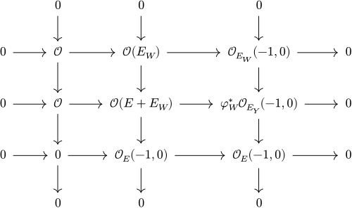
Applying the nine-lemma then gives us the desired short exact sequence from the rightmost column, and running the argument with the appropriate line bundle twist gives us the sequence for
The remaining morphisms in the tables are an immediate consequence of these distinguished triangles and the following statements:
which follow using the usual distinguished triangle (2.3) for
where we have used that and invoked equation (2.6) in order to compute cohomology of line bundles on the ruled surface
4.3.2. Morphisms between objects in the exceptional sequence. We summarise the results in Table 4.
where are objects in the exceptional sequence.
4.3.2.1. Morphisms to To begin, we see that
and that there are no morphisms in any other degree. One sees, since the map is induced by a transversal intersection at a single point, that the same result holds for for any choice of Since the objects are orthogonal to for any we find that for any
4.3.2.2. Morphisms to For each using that we obtain that
Since we must also have that Finally, using that we find that
4.4. Mutating the semiorthogonal decomposition
We are now in a position to perform the mutations described previously. The first set is defined by the following exact triangles:
We have that the objects are sheaves supported on Now note that the orthogonality of with implies that there is an isomorphism
which we obtain by applying to the triangle (4.8). This isomorphism is obtained by precomposing with so we obtain a commuting triangle.
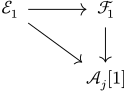
where the first non-zero map is an isomorphism due to the above commuting triangle. Hence, we have The next set of mutations is therefore defined by the following exact triangles:
We now have the job of tidying up the exceptional sequence
Lemma 4.10.
We have that
and if then we have that
Proof.
Applying to (4.11) gives an isomorphism
since Similarly, applying to (4.9) gives a long exact sequence of groups
which reads
Then, the map is non-zero, due to the fact that the extension of by is induced by the intersection of with and there is a map which is non-vanishing in a neighbourhood of the intersection locus, which is a reducible curve.
The second part of the lemma amounts to showing that the map
induced by precomposing with is non-zero. By mutating over and then we see that this is equivalent to showing that the map
is non-zero, where and the morphism is given by shifting and then precomposing with The argument to show that this map is non-zero is analogous to the one in the previous paragraph.
We use the above lemma to create the following distinguished triangles defining an object :
This object has a more explicit description.
Lemma 4.11.
Let be the object defined by the extension
Then, is given by the extension
Proof.
Since is orthogonal to we have giving us an extension
It is clear by applying to this short exact sequence that Next, we apply to the triangle (4.14) defining This gives an exact sequence
The claim is that the middle map is an isomorphism, so that But this is clear geometrically, since the extensions and are induced by the intersection of and and in a neighbourhood of the intersection point is precisely the identity. Hence, so we get that
Since there are no morphisms from or to we see that
Hence, It is clear by the mutations relating to that Hence, it suffices to show that We know that
and by similar reasoning as we did to show that the map is non-zero, we also find that the map
is non-zero. Hence, and since it follows immediately that
Next we mutate the object
Lemma 4.12.
We have that
and if then
Proof.
The first statement holds because of the exact triangle
and the fact that are orthogonal to For the second statement, we use the nine-lemma for derived categories, Lemma 2.2, and find that there is a distinguished triangle
We similarly define the object
The cone on the morphism is seen to be by another application of the derived nine-lemma. In particular, is not a sheaf.
Recall that we know that and an easy corollary of Lemma 4.9 is that The next lemmas will allow us to describe what happens if we pushforward the objects
Lemma 4.13.
For each the objects and are related by the exact triangle
where is given by the non-trivial extension
Proof.
Consider the exact triangles
Here, we use that where the first isomorphism is induced by postcomposing with and the second isomorphism is induced by postcomposing with Therefore, the map is a composition of the maps and and we can use the octahedral axiom to obtain an exact triangle
The triangle is non-split since the morphism in the triangle is the composition and we know that composing with induces an isomorphism
It is geometrically easier to see what happens if we first pushforward to the next lemma shows that the kernel of this contraction is simply generated by and We can see this as a direct consequence of the fact that for a surface node, the kernel of the contraction is generated by the pushforward of the bundle on the exceptional curve.
Lemma 4.14.
The kernel of the contraction is generated by
Proof.
Let be the reduced singular locus. Since the objects generate the kernel of the contraction we want to show that the kernel of is generated by the pushforwards of these objects. We use [15
A. Kuznetsov and E. Shinder, Categorical absorptions of singularities and degenerations. Épijournal Géom. Algébrique (2024), article no. 12, 42 pp., (Special volume in honour of Claire Voisin) Zbl 1545.14026 MR 4698898
, Theorem 5.2] to show this, which requires us to show thatwhere is the ideal sheaf of We can work in a neighbourhood of but locally near we find that is just for a nodal surface and that is, locally around the pullback of the resolution of that is, we have a pullback square.
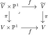
Let be the contraction, the exceptional curve and the nodal point. The desired result follows from pulling back the corresponding equivalence for which was shown in [15
A. Kuznetsov and E. Shinder, Categorical absorptions of singularities and degenerations. Épijournal Géom. Algébrique (2024), article no. 12, 42 pp., (Special volume in honour of Claire Voisin) Zbl 1545.14026 MR 4698898
, Corollary 5.6]and using flat base change
as needed.
Consider the extension on
so that is the skyscraper sheaf along the non-reduced branch
Lemma 4.15.
We have that
Proof.
Firstly, we see that is orthogonal to the objects for all Since
we immediately have We also know that
that is, the map factors through Then, applying the functor to the triangle gives us an exact sequence
which gives us that It follows then that for all integers and hence by Serre duality that also.
Now, we pushforward to Here, we have a distinguished triangle
One sees that is the bundle on the strict transform of The extension is non-split, since we showed that is orthogonal to so for example we know that has no endomorphisms in non-zero degrees. Hence, is the bundle on the strict transform of Now we can see that is the bundle on or equivalently,
Proof of Theorem 4.8.
To prove that
recall the defining triangle for (4.10)
In fact, we note that the transverse intersection of with along induces an extension between and By uniqueness, we find that is the pushforward of a line bundle on which is on on and on One verifies that this is a valid line bundle on the union since all restrictions to intersections agree. There is a line bundle on (i.e., the union of the reduced branches) which restricts to on and on We denote by the pushforward of this into Then, one sees that Let be the skyscraper sheaf along the reduced branch. Then,
Next, there is a unique extension in between and
We can consider the following triangle, obtained by pushing forward:
If this pushforward is non-split, it corresponds to the triangle obtained by embedding (4.18) using To show that it does not split, we pushforward the triangle
which must correspond to an extension in between and by Lemma 4.15. Then, one computes that there is indeed an extension induced by intersection
so that can only be A similar argument shows
Now let
The statement
follows from the fact that the cones on the morphisms and are in the kernel of so the image of under is contained within our absorbing category Combined with the fact that pushforward to and respectively, we find that the image of under is in fact the entire absorbing category and the desired equivalence follows from Bondal–Orlov localisation (see Section 2.1.5).
4.5. Structure of the categorical resolution
Having found the subcategory we now endeavour to describe the morphisms between the objects and how they behave under composition. Since the subcategory is found by mutating an exceptional sequence, the resulting objects also form an exceptional sequence
We recall that the objects are sheaves supported on the exceptional loci as defined in equation (4.6), while and are defined by the triangles induced by mutation given in equations (4.16), (4.17) and equations (4.12), (4.13), respectively.
4.5.1. Morphisms in the categorical resolution.
Theorem 4.16.
The morphisms in are described as follows:
- (1);
- (2);
- (3);
- (4).
The first claim of the theorem has already been proven in Section 4.3.2, and we prove the rest in a series of lemmas.
Lemma 4.17.
We have that and
Proof.
Apply to (4.15). Since we find that
and this gives us that
Applying to the triangle (4.14) defining we find that because we have
Then, applying to the triangle (4.15) gives us that
for and
Lemma 4.18.
We have that
Proof.
Applying to the exact triangle
and using the fact that we get the first statement. The second statement is proven by instead applying but now using that
4.5.2. Algebra structure of the categorical resolution. We now investigate how the compositions behave in the categorical resolution. Notice that for a object we have
and that we can recover the vector spaces of morphisms between objects in our categorical resolution as truncations of this algebra:
Subsequently, for any two objects in the exceptional sequence, we think of an element of as lifting some element of Since is a polynomial ring with no relations, this suggests the following.
Proposition 4.19.
All compositions in are non-zero.
Before proving the proposition, we illustrate some consequences. Let be non-zero degree 0 maps and be non-zero degree maps as described by the following quiver.
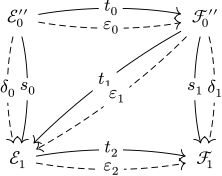
Letting denote the composition a corollary of Proposition 4.19 shows that up to rescaling, we can obtain the following relations:
Defining and we also see that
We can then extend to find bases of and of respectively.1 We can then visualise the category through the following quiver, where we omit compositions in non-zero degrees, the solid arrows are maps of degree the dashed arrows are maps in degree and the dotted arrows are maps in degree
Note that we can choose such that either of the relations or hold. However, it is not clear whether we can choose such that both commutativity relations simultaneously hold.
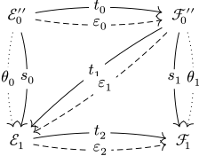
In particular, we highlight how our resolving category is essentially built out of the graded Kronecker quivers (see Definition 2.6) that resolve objects.
The proof of Proposition 4.19 comprises the remainder of the section through a series of lemmas.
4.5.2.1. Compositions with source
Lemma 4.20.
The compositions
are non-zero.
Proof.
The first statement follows from the proof of Lemma 4.17, which shows that the degree 0 map factors as The degree map similarly factors as
Lemma 4.21.
The composition is non-zero.
Proof.
We deduce that so we can immediately see that the composition is non-zero.
Lemma 4.22.
The composition is non-zero.
Proof.
Consider the following diagram.
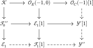
There is a unique degree morphism (up to scaling) and one can quickly show that this factors through both and by applying to the triangles defining and respectively. Hence, by the derived nine-lemma, we can complete along the dashed arrows to obtain exact triangles. The bottom-left square must then commute, so it follows that the map is non-zero and hence we find that Then, we have an exact triangle
We see that
and
and there are no morphisms in any other degrees. Then, applying to the triangle
we see that since that the map is an injection and hence the composition is non-zero.
4.5.2.2. Compositions with source and target
Lemma 4.23.
The compositions
are non-zero.
Proof.
Consider the exact triangle
and apply the functor. Using the fact that is orthogonal to and the defining exact triangle for
we find that
It follows that there is an isomorphism
so that the composition is non-zero, and similarly
so the composition is non-zero. We can also consider the exact triangle
and apply the functor. Using that we find an isomorphism
which implies that the composition is non-zero.
Lemma 4.24.
The composition is non-zero.
Proof.
Suppose for a contradiction that the composition is zero. Applying to the triangle
gives us an exact sequence
so that we have an isomorphism Hence, the left triangle commutes in the following diagram.
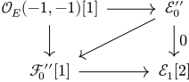
Since the right triangle commutes by assumption, it suffices to show that the composition
is non-zero, since then we obtain a contradiction. For this, we consider the non-split extension
and we only need to show that since then the map
is an injection, and hence the composition (4.20) is non-zero. Recall that diagram (4.19) gives us an exact triangle
There are no morphisms from to and in degree Hence,
and since we have our desired result.
4.5.2.3. Compositions with source and target
Lemma 4.25.
For all precomposing with induces isomorphisms
and postcomposing with induces isomorphisms
Proof.
Firstly, applying to the triangle
induces isomorphisms by precomposing with for Similarly, using that and then applying to the triangle (4.8)
gives us isomorphisms
for by composing with
Lemma 4.26.
Precomposing with induces an isomorphism
and postcomposing with induces an isomorphism
Proof.
By applying to
and using the results above, we find Then, we apply the functor to the same triangle and see that can only be non-zero in degrees Hence, applying to the triangle
we find that By applying to (4.21), we obtain an isomorphism
This shows the first statement.
We use a similar argument for the second statement. Consider the non-split extension
and apply We see that if then there is an isomorphism
We use the following diagram where the top-left square commutes, and so we complete the dashed arrows to exact triangles using the derived nine-lemma.
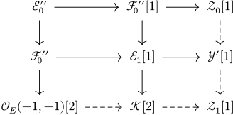
One quickly sees that and are only non-zero in degree and hence for From the previous calculations, we have that Hence, we find that by using the triangle
5. Deformation absorption through objects
In this section, we return to the singular curve defined in equation (3.1) and briefly discuss an interesting example of how objects behave when smoothing the curve. Our goal is to investigate whether these objects provide deformation absorptions, as described in Section 2.3.2. For this section, we recall the semiorthogonal decomposition (3.2)
We will denote for this section. For our purposes, we will define a smoothing of to be a flat family of curves where is a smooth pointed curve, the central fibre is and all other fibres are smooth. Note that we do not require the total space to be smooth.
Consider the surface
with the natural map We can embed into a projective bundle
so that the space is nodal, and the fibre over is given by
which is isomorphic to the curve Note that the generic fibre is a copy of so that is a smoothing of
Proposition 5.1.
The object provides a deformation absorption with respect to the smoothing
Proof.
The blow-up formula shows that there is a semiorthogonal decomposition
If is the inclusion, then is precisely the object generating the admissible subcategory of
It is not clear whether the object provides a universal deformation absorption, that is, whether the pushforward of generates an admissible category for all smoothings of We note that in our example, the pushforward of the object gives a object on which absorbs the singularities of the total space of the smoothing. One observes that the total space of a smoothing of cannot itself be smooth, for purely homological reasons. Indeed, consider the object The triviality of the normal bundle of in gives us the distinguished triangle using equation (2.3)
In the case that is the zero map, it is clear that is not in since is not in Otherwise, applying to the triangle shows that
for all which implies is not perfect. Hence, for another smoothing, we may similarly require that absorbs the singularities of the total space.
Acknowledgements
The author would like to thank his PhD supervisor Ed Segal for invaluable guidance throughout the project, and the anonymous reviewer for helpful comments which improved the paper.
Footnotes
- 1Note that we can choose such that either of the relations or hold. However, it is not clear whether we can choose such that both commutativity relations simultaneously hold.
References
- [1] A. Bondal, M. Kapranov, and V. Schechtman, Perverse schobers and birational geometry. Selecta Math. (N.S.) 24 (2018), no. 1, 85–143 Zbl 1436.14037 MR 3769727
- [2] A. Bondal and D. Orlov, Semiorthogonal decomposition for algebraic varieties. 1995 arXiv:alg-geom/9506012v1
- [3] A. Bondal and D. Orlov, Derived categories of coherent sheaves. In Proceedings of the International Congress of Mathematicians, Vol. II (Beijing, 2002), pp. 47–56, Higher Ed. Press, Beijing, 2002 Zbl 0996.18007 MR 1957019
- [4] A. I. Bondal, Representation of associative algebras and coherent sheaves (in Russian). Izv. Akad. Nauk SSSR Ser. Mat. 53 (1989), no. 1, 25–44. English translation. Math. USSR-Izv. 34 (1990), no. 1, 23–42 Zbl 0692.18002 MR 0992977
- [5] T. Bridgeland, Flops and derived categories. Invent. Math. 147 (2002), no. 3, 613–632 Zbl 1085.14017 MR 1893007
- [6] A. I. Efimov, Homotopy finiteness of some DG categories from algebraic geometry. J. Eur. Math. Soc. (JEMS) 22 (2020), no. 9, 2879–2942 Zbl 1478.14010 MR 4127943
- [7] D. Huybrechts, Fourier–Mukai transforms in algebraic geometry. Oxford Math. Monogr., Oxford University Press, Oxford, 2006, 307 pp. Zbl 1095.14002 MR 2244106
- [8] J. Karmazyn, A. Kuznetsov, and E. Shinder, Derived categories of singular surfaces. J. Eur. Math. Soc. (JEMS) 24 (2022), no. 2, 461–526 Zbl 1493.14023 MR 4382477
- [9] Y. Kawamata, On the derived category of a weighted projective threefold. Boll. Unione Mat. Ital. 15 (2022), no. 1–2, 245–252 Zbl 1492.14028 MR 4390551
- [10] Y. Kawamata, Semi-orthogonal decomposition of a derived category of a 3-fold with an ordinary double point. In H. Abban, G. Brown, A. Kasprzyk, and S. Mori (eds.), Recent developments in algebraic geometry. To Miles Reid for his 70th birthday, pp. 183–215, London Math. Soc. Lecture Note Ser. 478, Cambridge University Press, Cambridge, 2022 Zbl 1524.14040 MR 4480569
- [11] B. Keller, Derived categories and tilting. In L. A. Hügel, D. Happel, and H. Krause (eds.), Handbook of tilting theory, pp. 49–104, London Math. Soc. Lecture Note Ser. 332, Cambridge University Press, Cambridge, 2007 MR 2384608
- [12] A. Kuznetsov, Lefschetz decompositions and categorical resolutions of singularities. Selecta Math. (N.S.) 13 (2008), no. 4, 661–696 Zbl 1156.18006 MR 2403307
- [13] A. Kuznetsov, Base change for semiorthogonal decompositions. Compos. Math. 147 (2011), no. 3, 852–876 Zbl 1218.18009 MR 2801403
- [14] A. Kuznetsov and V. A. Lunts, Categorical resolutions of irrational singularities. Int. Math. Res. Not. IMRN 2015 (2015), no. 13, 4536–4625 Zbl 1338.14020 MR 3439086
- [15] A. Kuznetsov and E. Shinder, Categorical absorptions of singularities and degenerations. Épijournal Géom. Algébrique (2024), article no. 12, 42 pp., (Special volume in honour of Claire Voisin) Zbl 1545.14026 MR 4698898
- [16] A. Kuznetsov and E. Shinder, Derived categories of Fano threefolds and degenerations. Invent. Math. 239 (2025), no. 2, 377–430 Zbl 1564.14091 MR 4850600
- [17] J. P. May, The additivity of traces in triangulated categories. Adv. Math. 163 (2001), no. 1, 34–73 Zbl 1007.18012 MR 1867203
- [18] D. O. Orlov, Projective bundles, monoidal transformations, and derived categories of coherent sheaves (in Russian). Izv. Ross. Akad. Nauk Ser. Mat. 56 (1992), no. 4, 852–862. English translation. Russ. Acad. Sci. Izv. Math. 41 (1993), no. 1, 133–141 Zbl 0798.14007 MR 1208153
- [19] D. O. Orlov, Triangulated categories of singularities and D-branes in Landau–Ginzburg models (in Russian). Tr. Mat. Inst. Steklova 246 (2004), 240–262. English translation. Proc. Steklov Inst. Math. 246 (2004), 227–248 Zbl 1101.81093 MR 2101296
- [20] N. Pavic and E. Shinder, theory and the singularity category of quotient singularities. Ann. K-Theory 6 (2021), no. 3, 381–424 Zbl 1490.14020 MR 4310324
- [21] N. Pavic and E. Shinder, Derived categories of nodal del Pezzo threefolds. Taiwanese J. Math. 29 (2025), no. 6, 1607–1632 Zbl 08150207 MR 5003266
- [22] F. Xie, Nodal quintic del Pezzo threefolds and their derived categories. Math. Z. 304 (2023), no. 3, article no. 48, 28 pp. Zbl 1528.14022 MR 4610379
Cite this article
Aporva Varshney, Categorical absorption of a non-isolated singularity. J. Noncommut. Geom. 20 (2026), no. 4, pp. 1419–1464
DOI 10.4171/JNCG/684